Species Table - Specific Heat (Cp)

Navigation: User Guide ➔ Species Table ➔ Specific Heat (Cp)

Main	Editing User Species Database		Species Database Data Table - Theory and Equations								Viewing Properties
Species Database	Editing User Species Database	Importing data into Species Database	Species Table	Heat of Formation and Entropy	Density	Specific Heat (Cp)	Phase Change (solubility)	BPE & Acid/Base Ka/b	Vapour Properties	Transport Properties	Viewing Species Properties	Species Properties Reports

---

Introduction

By selecting a Cp equation, together with H25 and S25, we are defining the equations to be used for thermodynamic calculations Cp, Enthalpy and Entropy. The main calculation used in SysCAD is Enthalpy.

The Cp field is optional, but if it is left blank it will have the following consequences: Estimation of Specific Heat for Mineral Species

Discussion Page Estimation of Specific Heat for Mineral Species

• SysCAD will assume a constant value:

  For solids and gases, SysCAD will assume a value of 1.0 kJ/kg.K,

  For liquids, SysCAD will assume a value of 2.0 kJ/kg.K.

  This assumption will be shown as a warning in the message window when loading a project.

• If the species is used in a Reaction then the user will either:

  Have to define the Heat of Reaction (HOR) manually in the reaction file; or

  Receive a warning that Cp is not defined in the database.

  See Reaction Block (RB) for further information on reactions. (This is because Cp is used to calculate heats of reaction for chemical reactions specified in SysCAD

Notes:

1. The unit for Heat Capacity is J/mol.K.
2. All Cp equations must use temperature in degrees Kelvin (K). If you have a Cp relation expressed in terms of degrees Centigrade or Fahrenheit it will need to be converted to a function of degrees Kelvin.
3. Valid Cp equations must be supplied for all species used in the project to obtain a correct energy balance in SysCAD.
4. For Cp, when the temperature is outside of the specified temperature range, then a constant value for Cp at the temperature limit is used.
5. The integral of Cp gives H (Enthalpy) equation. The Cp equations are integrated over a temperature range to obtain the change of enthalpy around a unit operation.

   [math]\displaystyle{ \Delta H = \int\limits_{T_1}^{T_2}Cp dT\, }[/math]

   Where T1 is Initial temperature and T2 Final temperature

6. The enthalpy calculation when the species is outside of the defined temperature ranges is calculated using the Cp at the limit of the defined temperature range:
   • If T₁ < T_{Lower Limit} then:

   [math]\displaystyle{ \Delta H _{T_1 \; \to \; T_{lowerlimit}} \quad = Cp_{T_{lowerlimit}} \quad *\left ( T_{lowerlimit} - T_1 \right)\, }[/math]

   • Similarly, if T₂ > T_{Upper Limit} then:

   [math]\displaystyle{ \Delta H _{T_{upperlimit} \quad \; \to \; T_2} \; = Cp_{T_{upperlimit}} \quad *\left ( T_2 - T_{upperlimit} \right)\, }[/math]

7. The integral of H (Enthalpy) gives S (Entropy) equation.

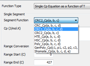
The user may choose from a number of different functions for the Cp value, as shown in the image below:

Each of these will be described in the sections below:

Constant Cp value

The first 2 functions represent constant Cp values:

• Constant Value; and
• Constant Value with Temperature Range.

With these 2 options Cp does not vary as a function of temperature. However, with the option that includes a Range, the user may define a specific temperature range for the value.

Cp Equation Format (Single or Multi segment)

The user may define a single temperature range for the Cp value, SingleSegment, OR multiple temperature ranges, MultiSegment. In both cases, the Cp equations that are used have the same form, which are described further on in this section.

Single Segment

If the user selects 'SingleSegment' then they need only enter a single Cp equation and the range for that equation. The form of the equation can be any of those shown below.

The forms of the equations are explained in the sections below.

Multi Segment

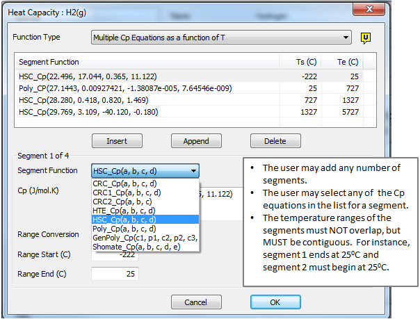
If the user selects 'MultiSegment':

1. They may enter a number of Cp equations covering different temperature ranges.
2. Each Cp equation must be specified with the temperature range for which it is valid.
3. Temperature ranges MUST NOT overlap.
4. Temperature ranges MUST be contiguous, i.e. there must not be any gaps in the temperature ranges.
5. Different forms of the Cp equation can be used for different temperature ranges.

See the example below:

To insert a new equation before the first equation, select the first equation and press the Insert button.

To insert a new equation after the last equation, press the Append button.

To insert a new equation inbetween current equations, select the nearest equation and press the Insert button. An additional equation with the same parameters will be added after the selected equation. The previous temperature range for the selected equation will be split equally over the selected and new equation.

Cp Equation Format

The format for the Cp equation and corresponding Temperature Range is the same if the user has chosen single or multi segment. The format is as follows:

Cp Equation Name(a,b,...):Range(C or K, T_L, T_H)

Where:

1. Each Cp Equation is described below (Note: The equation always uses K)
2. The Range is the temperature range for which the Cp equation is valid -
   • The range can be given in degrees Celsius (C) or Kelvin (K) (Note: While the range can be given in C or K, the actual Cp equation always uses K).
   • T_L is the Lowest temperature at which the Cp equation is valid. The minimum allowed value is 1K.
   • T_H is the Highest temperature at which the Cp equation is valid.

By selecting a Cp equation, the corresponding Enthalpy and Entropy equations are selected. The available Cp equation formats are given below.

NOTES

1. All temperatures in the above formulae are in Kelvin. It does not matter if you give the range in units of C, K or F, the correlation, must use K.
2. If you want to use a correlation for Cp that is given as a function of C or F, set up a spreadsheet to generate the data for the range you want and then curve fit the data in degrees K and enter that into SysCAD (NB you should be able to reproduce an exact fit of your original correlation).

Refer to Stream Specific Heat values (Cp) for an example of how these individual heat capacities are used to determine the heat capacity of a stream.

Cp Equation Format	Function format in Species Table	Equation	Notes
CRC Equation	CRC_Cp(a,b,c,d)	[math]\displaystyle{ C_p = a + b.10^{-3} \, T + \dfrac{c.10^5}{T^2} + d.10^{-6} \, T^2\, }[/math]	T - Temperature in K
CRC Equation (alternative format 1)	CRC1_Cp(a,b,c,d)	[math]\displaystyle{ C_p = a + b.10^{-3} \, T + c.10^{-6} \, T^2 + \dfrac{d.10^5}{T^2}\, }[/math]	T - Temperature in K
CRC Equation (alternative format 2)	CRC2_Cp(a,b,c)	[math]\displaystyle{ C_p = MolecularWeight \times \left( a + b.T - \dfrac{c}{T^2} \right)\, }[/math]	T - Temperature in K
HTE Equation format	HTE_Cp(a,b,c,d)	[math]\displaystyle{ C_p = 4.186 \times \left(b + 2*c.10^{-3} \, T - \dfrac{d.10^5}{T^2}\right)\, }[/math]	T - Temperature in K The first parameter a is required but is not used in the HTE equation and is ignored by SysCAD.
HSC Equation format	HSC_Cp(a,b,c,d)	[math]\displaystyle{ C_p = a + b.10^{-3} \, T + \dfrac{c.10^5}{T^2} + d.10^{-6} \, T^2\, }[/math]	T - Temperature in K This equation is the same as the CRC_Cp format 1 equation.
HSC_2 Equation format (Available from Build 139.)	HSC2_Cp(a,b,c,d,e,f)	[math]\displaystyle{ C_p = a + b.10^{-3} \, T + \dfrac{c.10^5}{T^2} + d.10^{-6} \, T^2 + \dfrac{e.10^8}{T^3} + f.10^{-9} \, T^3 \, }[/math]	T - Temperature in K a, b, c, d, e and f are coefficients estimated from experimental data. This is an extended HSC_Cp equation with two extra terms. This equation is for importing from HSC8 or newer with more than 4 terms.
Polynomial Equation format	Poly_Cp(a,b,c,d,e)	[math]\displaystyle{ C_p = a + bT + cT^2 + dT^3 + eT^4\, }[/math]	T - Temperature in K The Poly_Cp will support upto 5 terms, user can ignore the later constants if the polynomial has lesser terms. For example: For Cp = 28.5 + 0.04T + 0.01T^2, use Poly_Cp(28.5,0.04,0.01)
General Polynomial Equation format	GenPoly_Cp(c1,p1,c2,p2,c3, p3,c4,p4,c5,p5,...)	[math]\displaystyle{ C_p = c_1 T^{p_1} + c_2 T^{p_2} + c_3 T^{p_3} + c_4 T^{p_4} + c_5 T^{p_5}\dots\, }[/math]	T - Temperature in K This equation can have any number of terms, so the parameters are optional. You only need to enter as many parameters as are needed. For Polynomials with 5 terms or less, we recommend using the Polynomial Equation format (Poly_Cp) format.
Shomate Equation	Shomate_Cp(a,b,c,d,e)	[math]\displaystyle{ C_p = a + b.10^{-3} \, T + c.10^{-6} \, T^2 + d.10^{-9} \, T^3 + \cfrac{e.10^6}{T^2}\, }[/math]	T - Temperature in K The Shomate Equation is used for many applications. Data can be obtained from NIST Chemistry WebBook. An example is to fit data from the NIST web site for gas components with higher temperature ranges. e.g. Oxygen
NASA Glenn Coefficients Equation	NASAGlenn_Cp(a1,a2,a3,a4, a5,a6,a7,b1,b2)	[math]\displaystyle{ \cfrac{C_p(T)}{R} = a_1 \, T^{-2} + a_2 \, T^{-1} + a_3 + a_4 \, T + a_5 \, T^2 + a_6 \, T^3 + a_7 \, T^4\, }[/math]	[math]\displaystyle{ C_p(T)\, }[/math] - molar heat capacity at constant pressure at temperature T for standard state T - Temperature in K, R - universal gas constant 8.314510 J/(mol.K),b1 - integration constant for enthalpy, b2 - integration constant for entropy H25 and S25 can be calculated directly using this equation. It is therefore recommended to specify "FromCp()" in fields for H25 and S25. If user specifies a value for H25 (or S25) and this does not match calculated value an error is given. The NASA Glenn Coefficients Equation is used by the NASA Glenn computer program CEA (chemical Equilibrium with Applications). The NASA Data can be obtained from http://www.grc.nasa.gov/WWW/CEAWeb/.
General Gibbs Equation format	Gibbs_Cp(a, b, c, d, e, f)	[math]\displaystyle{ C_p(T) = -c - 2 \, dT - 6e \, T^2 - \dfrac{2f}{T^2} }[/math] The Cp equation above is derived from the Gibbs function: [math]\displaystyle{ G(T) = a + bT + cT.\ln(T) + dT^2 + eT^3 + \dfrac{f}{T} }[/math] The formula for absolute enthalpy is: [math]\displaystyle{ H(T)=a-cT-dT^2-2eT^3+2\frac{f}{T} }[/math]	T - Temperature in K The basic Gibbs function for constant pressure is G = H - TS, where H is Enthalpy and S Entropy. H25 and S25 can be calculated directly using this equation. It is therefore recommended to specify "FromCp()" in fields for H25 and S25. If user specifies a value for H25 (or S25) and this does not match calculated value an error is given.
General Gibbs Equation format 2 (Available from Build 139.)	Gibbs2_Cp(a, b, c, d, e, f)	[math]\displaystyle{ C_p(T) = -c - 2dT - \dfrac{2e}{T^2} - \dfrac{6f}{T^3} }[/math] The Cp equation above is derived from the Gibbs function: [math]\displaystyle{ G(T) = a + bT + cT\ln(T) + dT^2 + \dfrac{e}{T} + \dfrac{f}{T^2} }[/math]	T - Temperature in K The basic Gibbs function for constant pressure is G = H - TS, where H is Enthalpy and S Entropy. H25 and S25 can be calculated directly using this equation. It is therefore recommended to specify "FromCp()" in fields for H25 and S25. If user specifies a value for H25 (or S25) and this does not match calculated value an error is given.
Gibbs with Magnetic Ordering Equation format (Available from Build 139.33612.)	GibbsMag_Cp(a,b,c,d,e,f, p, B0, TC (or TN))	General Gibbs Equation format is modified to add magnetic ordering term: [math]\displaystyle{ G(T) = a + bT + cT.\ln(T) + dT^2 + eT^3 + \dfrac{f}{T} + G^{mag}(T) }[/math] [math]\displaystyle{ G^{mag}(T) \left[\frac{J}{mol} \right] = RT\ln(B_0+1)g(\tau) }[/math] [math]\displaystyle{ \tau = \frac{T}{T_C} }[/math] [math]\displaystyle{ g(\tau) = \begin{cases} 1-\left[\frac{79\tau^{-1}}{140p}+\frac{474}{497}\left(\frac{1}{p} -1 \right)\left(\frac{\tau^{3}}{6}+\frac{\tau^{9}}{135}+\frac{\tau^{15}}{600} \right) \right]/D & \text{if } \tau \leq 1 \\ -\left[\frac{\tau^{-5}}{10}+\frac{\tau^{-15}}{315}+\frac{\tau^{-25}}{1500} \right]/D & \text{if } \tau \gt 1 \end{cases} }[/math] [math]\displaystyle{ D=\frac{518}{1125}+\frac{11692}{15975}\left(\frac{1}{p} -1 \right) }[/math]	This functions adds magnetic ordering parameters to Gibbs_Cp function above. T - Temperature in K B0 is average magnetic moment per atom [math]\displaystyle{ \tau }[/math] is critical temperature TC is Curie temperature for ferromagnetic materials TN is Neel temperature for antiferromagnetic materials [math]\displaystyle{ p }[/math] represents the fraction of magnetic enthalpy absorbed above the critical temperature. Typically [math]\displaystyle{ p }[/math] is 0.4 or 0.28 When multiple temperature segments are entered, the magnetic ordering parameters should be identical for each temperature segment. Cp, H and S functions are derived from Gibbs function with magnetic ordering parameters. H25 and S25 can be calculated directly using this equation. It is therefore recommended to specify "FromCp()" in fields for H25 and S25. If user specifies a value for H25 (or S25) and this does not match calculated value an error is given.
Gibbs Extended Equation format (Available from Build 139.33612.)	GibbsEx_Cp(a,b,c,d,e,f, P1,E1,P2,E2,P3,E3, P4,E4, P5,E5,P6,E6)	[math]\displaystyle{ C_p(T) = -c - 2dT - 6eT^2 - \dfrac{2f}{T^2} + \sum\nolimits P_{i}E_{i}T^{E_{i}-1}(1-E_{i}) + \dfrac{P_{lg}}{T} }[/math] The Cp equation above is derived from the Gibbs function: [math]\displaystyle{ G(T) = a + bT + cT.\ln(T) + dT^2 + eT^3 + \dfrac{f}{T} + \sum\nolimits P_{i}T^{E_{i}} + P_{lg}\ln T }[/math]	T - Temperature in K The basic Gibbs function for constant pressure is G = H - TS, where H is Enthalpy and S Entropy. H25 and S25 can be calculated directly using this equation. It is therefore recommended to specify "FromCp()" in fields for H25 and S25. If user specifies a value for H25 (or S25) and this does not match calculated value an error is given. This function is an extension of Gibbs_Cp with between 1 and 6 optional pairs of parameters Pi and Ei. Parameters P2 and E2 and later are optional and can be omitted. If Ei = 99, the corresponding Pi is interpreted as a logarithmic term, Plg. There can only be one logarithmic term.
Gibbs Extended with Magnetic Ordering Equation format (Available from Build 139.33612.)	GibbsExMag_Cp(a,b,c,d,e,f, P1,E1,P2,E2,P3,E3, P4,E4, P5,E5,P6,E6, p, B0, TC (or TN))	Extended Gibbs Equation format is modified to add magnetic ordering term: [math]\displaystyle{ G(T) = a + bT + cT.\ln(T) + dT^2 + eT^3 + \dfrac{f}{T} + \sum\nolimits P_{i}T^{E_{i}} + P_{lg}\ln T + G^{mag}(T) }[/math] [math]\displaystyle{ G^{mag}(T) \left[\frac{J}{mol} \right] = RT\ln(B_0+1)g(\tau) }[/math] [math]\displaystyle{ \tau = \frac{T}{T_C} }[/math] [math]\displaystyle{ g(\tau) = \begin{cases} 1-\left[\frac{79\tau^{-1}}{140p}+\frac{474}{497}\left(\frac{1}{p} -1 \right)\left(\frac{\tau^{3}}{6}+\frac{\tau^{9}}{135}+\frac{\tau^{15}}{600} \right) \right]/D & \text{if } \tau \leq 1 \\ -\left[\frac{\tau^{-5}}{10}+\frac{\tau^{-15}}{315}+\frac{\tau^{-25}}{1500} \right]/D & \text{if } \tau \gt 1 \end{cases} }[/math] [math]\displaystyle{ D=\frac{518}{1125}+\frac{11692}{15975}\left(\frac{1}{p} -1 \right) }[/math]	This functions adds magnetic ordering parameters to GibbsEx_Cp function above. T - Temperature in K B0 is average magnetic moment per atom [math]\displaystyle{ \tau }[/math] is critical temperature TC is Curie temperature for ferromagnetic materials TN is Neel temperature for antiferromagnetic materials [math]\displaystyle{ p }[/math] represents the fraction of magnetic enthalpy absorbed above the critical temperature. Typically [math]\displaystyle{ p }[/math] is 0.4 or 0.28 When multiple temperature segments are entered, the magnetic ordering parameters should be identical for each temperature segment. Cp, H and S functions are derived from Gibbs function with magnetic ordering parameters. H25 and S25 can be calculated directly using this equation. It is therefore recommended to specify "FromCp()" in fields for H25 and S25. If user specifies a value for H25 (or S25) and this does not match calculated value an error is given. This function is an extension of Gibbs_Cp with 6 additional pairs of parameters Pi and Ei, followed by the three magnetic ordering contribution terms p, B0, TC (or TN), for a total of 21 parameters. If Ei = 99, the corresponding Pi is interpreted as a logarithmic term, Plg. There can only be one logarithmic term.
Gibbs ChemApp Equation format	GibbsChemApp_Cp(a,b,c,d,e,f, P1,E1,P2,E2,P3,E3, P4,E4, P5,E5,P6,E6)	[math]\displaystyle{ C_p(T) = -c - 2dT - 6eT^2 - \dfrac{2f}{T^2} + \sum\nolimits P_{i}E_{i}T^{E_{i}-1}(1-E_{i}) + \dfrac{P_{lg}}{T} }[/math] The Cp equation above is derived from the Gibbs function: [math]\displaystyle{ G(T) = a + bT + cT.\ln(T) + dT^2 + eT^3 + \dfrac{f}{T} + \sum\nolimits P_{i}T^{E_{i}} + P_{lg}\ln T }[/math]	T - Temperature in K This equation is the same as the GibbsEx_Cp equation. The basic Gibbs function for constant pressure is G = H - TS, where H is Enthalpy and S Entropy. H25 and S25 can be calculated directly using this equation. It is therefore recommended to specify "FromCp()" in fields for H25 and S25. If user specifies a value for H25 (or S25) and this does not match calculated value an error is given. This function is an extension of Gibbs_Cp with between 1 and 6 optional pairs of parameters Pi and Ei. If Ei = 99, the corresponding Pi is interpreted as a logarithmic term, Plg. There can only be one logarithmic term.

Laliberté Cp Function

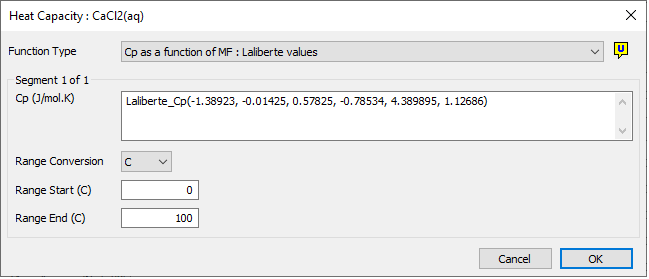
The user may choose to use the Laliberté method for calculating the specific heat of an aqueous species. This method uses the constants as calculated by Laliberté based on data obtained from many references.

The Standard "mass weighted mean" method for calculating the Cp (and Enthalpy) of a mixture is used, however for individual aqueous species using Laliberté Cp method there is a mass fraction term. All other individual aqueous and liquid phase species contribute to Cp of mixture in the normal way.

The aqueous solution specific heat is calculated using the water specific heat, Cp_w and the solutes heat capacity using following equation (which is simply the Standard mixture Cp calculation):

[math]\displaystyle{ Cp_m = m_wCp_w + \sum{m_iCp_i} }[/math]

The heat capacity of each solute in solution is calculated from:

[math]\displaystyle{ Cp_i= a_1e^{\alpha}+a_5(1-m_w)^{a_6} }[/math]

Where

[math]\displaystyle{ {{\alpha= a_2\times T +a_3e^{0.01T}+a_4(1-m_w)}} }[/math]

mw	=	mass fraction of water
mi	=	mass fraction of solute species i (i.e. all aqueous species only)
Cpw	=	Heat capacity of water (at stream temperature and pressure), kJ/kg.K
Cpi	=	Heat capacity of solute i, kJ/kg.K
Cpm	=	solution Heat capacity, kJ/kg.K
T	=	Temperature in °C
a1 to a6	=	dimensionless empirical constants for each solute species.

Entering the data into the database

The Laliberté equation constants can be entered into the Species Database directly (based on Cp in kJ/kg.K and temperature in °C), SysCAD will apply the conversions internally to convert the value into the required (J/mol.K).

For Example:

Notes

1. Important: This method does NOT include a calculation for Entropy.
2. The constants for most aqueous species are valid for temperatures between approximately 5 and 120°C.
3. If the unit temperature is outside of the species temperature range, then SysCAD will use the values at the temperature limit.
4. Although the published data has some maximum mass fraction data, in SysCAD implementation there are no limits applied or warnings given when outside of the fitted data mass fraction range.
5. The Enthalpy is calculated by numerical integration method. This iterative calculation can fail for some combination of constants.
6. The Enthalpy function is tested at species temperature limits at project load, and if calculation of enthalpy fails an error message is given and project will not load.
7. Water heat capacity is calculated in SysCAD as described here: Water and Steam Properties.
8. The user MUST define all 6 constants and also the valid range for the function.
9. To remove the temperature dependence, set a2 = 0 AND a3 = 0 (or a1 = 0).
10. Due to the method of solving for enthalpy, a2 = 0 is not allowed unless a3 = 0 or a1 = 0.
11. The mass fraction parameter used for calculation of individual solute species Cp is based on ALL aqueous species dissolved in the solution regardless of Cp method selected for the individual solute species.
12. This method is intended to calculate the Enthalpy of an aqueous solution taking into account some dependence on heat of mixing of the solution by use of the mass fraction term. Therefore, it is recommended that all aqueous species in a project use the Laliberté method for the results to be consistent with the reference data.

Reference

1. Laliberté M. A Model for Calculating the Heat Capacity of Aqueous Solutions, with Updated Density and Viscosity Data. J.Chem Eng. Data 2009.

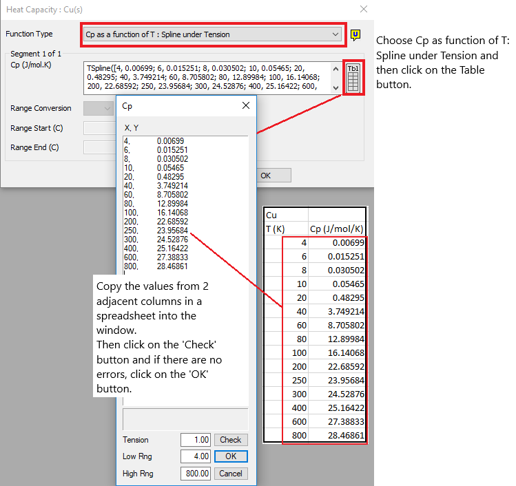
Cp as a Function of Temperature - Spline under Tension

Select this option if Cp varies as a function of Temperature and the user has data points for this. SysCAD will then use a Spline method to interpolate from the data in the table.

Notes:

1. Important: This method does NOT include a calculation for Entropy.
2. A spline is a special function defined piecewise by polynomials and is used in interpolating problems.
3. A fitted equation will be processed more quickly within SysCAD and hence is preferred to entering TSpline data.

Please refer to Entering Spline Data for more information.

See the example below:

Examples of Cp Equations

Species	Cp	Total Temperature Range (C)
CaCO3(s)	HTE_Cp(-9122, 23.8351, 3.2146, 5.1569):Range(C, 25, 927)	25 to 927
CO2(g)	Shomate_Cp(19.7961, 0.07344, -5.60221e-005, 1.71541e-008):Range(K, 298.15, 1000)	25 to 726.85
Fe2(SO4)3(aq)	Poly_Cp(-22429, 57.4101, 29.6643, 7.9582):Range(K, 298.15, 900)	25 to 626.85
2CaO*SiO2(s)	HSC_Cp(145.896, 40.752, -26.192, 0.000):Range(C, 25, 848), HSC_Cp(134.557, 46.108, 0.000, 0.000):Range(C, 848, 1439), Const(205.016):Range(C, 1439, 2130)	25 to 2130

Important Points about Cp

1. By selecting a Cp equation you are simultaneously selecting the related enthalpy and entropy equations.
2. When entering or reviewing Cp equations, H25 and S25 should be checked at the same time. Some Cp equation formats (e.g. NASAGlenn and Gibbs) calculate H25 and S25 directly from the Cp correlation parameters.
3. Heat capacity cannot be zero (except for special case of H+(aq), see below). Therefore, if the value in the species database is zero for a species in the project, SysCAD will not initialise and the user will see the following error message: Species:Bad Cp: Value too small = 0J/mol at T 5 C (where species is the actual species with the zero Cp). The database Cp parameters will need to be corrected before you will be able to continue with a project.
4. H+(aq) should have a heat capacity of zero.
5. Enthalpy MUST increase with temperature with the exception of AQUEOUS compounds. Therefore, if as a result of the values in the species database for the specified temperature range, a negative increase for Cp with temperature is calculated, SysCAD will not initialise and the user will see the following error message: Bad Enthalpy: msH decreases with T for species (where species is the actual species with the negative Cp). The database Cp parameters will need to be corrected before you will be able to continue with a project. For an aqueous compound, the Cp data can effectively be used as a correction factor for that compound in solution. The Cp equation for an aqueous species may not be intended to be valid for the compound in its pure state. To be recognised as an aqueous compound, the phase name must be "aq" or "a".