Python Example - Getting Started
Navigation: User Guide ➔ COM Automation ➔ Python Automation ➔ Example - Basic Usage
Basic Usage: Opening, running, setting and getting tags
This basic example opens up the Demo Gold steady state ProBal project, looks at the amount of gold in the product, changes the feed composition tag, runs the project, then looks at the new value of gold in product.
## Example Automation Using python.
import sys
import time
try:
  import win32com.client as wc    ## PyWin32 COM Client
except:
  print ("Win32 python extensions not found")
  print ("Install pywin32:  https://pypi.org/project/pywin32/")
  sys.exit(1)

ProgID = "SysCADSimulator93.Application"
SysCAD = wc.DispatchEx(ProgID)  ## Fire up SysCAD
build = SysCAD.VersionNumber(2) ## You can now query the build number

ScdDir = r'C:\SysCAD%d' % build
print ("Using Build", build, "Install Directory is ", ScdDir)

ScdPrj = r'\Examples\25 Gold\Demo Gold Project.spf\Project.spj'
#### If you use \ in file and directory strings use a raw string or escape \'s
#### e.g. Prj = SysCAD.OpenProject('C:\\SysCADProjectFiles\\Sample.spf\\Project.spj')
####    Prj = SysCAD.OpenProject('C:/SysCADProjectFiles/Sample.spf/Project.spj')  ## also works

Prj = SysCAD.OpenProject(ScdDir+ScdPrj)  ## Open project

Tags = Prj.Tags
#### The tag naming was changed in the distributed examples for 138
goldFlow = "P_007.Qo.QM.Au(s) (oz/d)"
print ("Gold in product", end=" ")
print (Tags.TagValue(goldFlow))  ## Get a tag value

Solver = Prj.Solver
ProBal = Solver.ProBal

ProBal.Start()                        ## Start ProBal
while True:                           ## Wait until solved
   print ("Solving...")
   time.sleep(.5)
   if ProBal.IsStopped:
       break
print ("Feed ppm in gold ore", Tags.TagValue("FEED_ppm_SET.TC[1].User.Value"))   ## Print another tag
print ("Changing value to 45 ppm")
Tags.SetTagValue("FEED_ppm_SET.TC[1].User.Value", 45)  ## Change tag value
ProBal.Start()          ## and re-solve
while True:
   print ("Solving...")
   time.sleep(.5)
   if ProBal.IsStopped:
       break
print ("Gold in product", end = " ")
print (Tags.TagValue(goldFlow))   ## Print the same tag

SysCAD.CloseProject(False)
##
time.sleep(5)
del(Solver)
del(Tags)
del(Prj)
del(SysCAD)
The output will be something like:
Using Build 138 Install Directory is  C:\SysCAD138
Gold in product 57.6095546633
Solving...
Feed ppm in gold ore 40.0
Changing value to 45 ppm
Solving...
Gold in product 64.8079746073
See Notes for general information and troubleshooting on using SysCAD COM with Python.
When using COM you create a number of COM objects representing various features of SysCAD: a Project object (Prj), a Tags object, a Solver object and so on. Keeping track of these (and cleaning up afterwards) is a mess, and we can simplify this by encapsulating all the functionality in a single python class which we will use for subsequent examples. We assume all the necessary packages are installed: if you get errors when importing a particular package such as numpy, you will need to install it to continue.
Encapsulating COM functionality in a python class
It is a good idea to create a python class which encapsulates all the functionality needed in once place. Once you have the class, you can reuse it. The syscadif.py module in the code in the link encapsulates basic SysCAD COM functionality in a python class SysCADCom, and we will use it in subsequent examples. You need to save this file either in the working directory (where the python script is located), or somewhere on your PYTHONPATH
Some methods
| Method | Description |
|---|---|
| sc = SysCADCom() | Create a SysCADCom class instance. |
| OpenProject(file) | Open a SysCAD project |
| CloseProject() | Close the current project |
| Close(): | Close SysCAD and clean up COM objects |
| getTag(str) | Get the value of tag str |
| setTag(str, val) | Get the value of tag str to val |
| getTags(tagLis) | Get the value of tags in list or iterable |
| setTags(tagLis, vals) | Set the value of tags in list to items in vals |
| run() | Run a Probal model |
| runScenarios(Vals, TagsIn, TagsOut) | Run scenarios setting a single or mutiple tags |
We also implement __getitem__ and __setitem__ methods for the class, so we can use shorthand notation similar to PGM for getting and setting tags:
flow = sc["P_007.Qo.QM.Au(s) (oz/d)"] ## or just flow = sc.getTag("P_007.Qo.QM.Au(s) (oz/d)") ##
sc["$Solver.Cmd.CompleteReset"] = 1  ## equivalent to sc.setTag("$Solver.Cmd.CompleteReset", 1)
Not all COM methods are implemented directly via the class but you still have access to these via the member attributes:
sc.SysCAD.CreateProject(cfg, prj) ## Create a new project
Using the SysCADCom class, the example in the first section now becomes
## Example Automation Using python.
import syscadif  ## SysCAD COM interface class

sc = syscadif.SysCADCom()
ScdDir = r'C:\SysCAD%d' % sc.build
print ("Using Build", sc.build, "Install Directory is ", ScdDir)
ScdPrj = r'\Examples\25 Gold\Demo Gold Project.spf\Project.spj'
sc.OpenProject(ScdDir+ScdPrj)  ## Open project
goldFlowTag = "P_007.Qo.QM.Au(s) (oz/d)"

sc.run()
print ("Feed ppm in gold ore", sc["FEED_ppm_SET.TC[1].User.Value"])   ## Print another tag
print ("Gold in product", sc[goldFlowTag])
input ("Hit any key to change a tag, model reset and rerun")
sc["$Solver.Cmd.CompleteReset"] = 1
print ("Changing value to 45 ppm")
sc["FEED_ppm_SET.TC[1].User.Value"] = 45  ## Change tag value
sc.run()          ## and re-solve
print ("Gold in product", sc[goldFlowTag])
input ("Hit any key to finish")

sc.CloseProject()
sc.Close()
Further Usage: Scenarios, plots, etc.
Running a series of scenarios
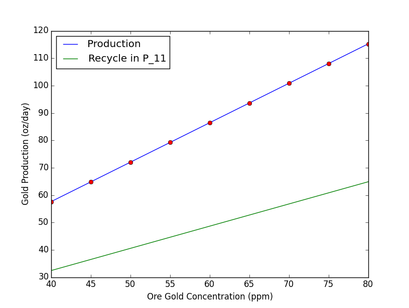
Extending on the first example, we can easily make plots:
The SysCADCom class has a useful function to run a series of scenarios and collect the values of any number of tags
import syscadif
import matplotlib.pyplot as plt

sc = syscadif.SysCADCom()
ScdDir = r'C:\SysCAD%d' % sc.build
ScdPrj = r'\Examples\25 Gold\Demo Gold Project.spf\Project.spj'

sc.OpenProject(ScdDir+ScdPrj)  ## Open project

X = list(range(40, 85, 5))  ## for Python3 since since range() is now a generator and we need to reuse X
Y = sc.RunScenarios(X, "FEED_ppm_SET.TC[1].User.Value", ["P_007.Qo.QM.Au(s) (oz/d)", "P_011.Qo.QM.Au(s) (oz/d)"])
Z = [y[0] for y in Y]  # flatten
Z1 = [y[1] for y in Y]
plt.plot(X, Z, label="Production")
plt.plot(X, Z, "ro")
plt.plot(X, Z1, label = "Recycle in P_11")
plt.xlabel("Ore Gold Concentration (ppm)")
plt.ylabel("Gold Production (oz/day)")
plt.legend(loc=2)
plt.show()

sc.CloseProject()
sc.Close()
Sensitivity Analysis Example
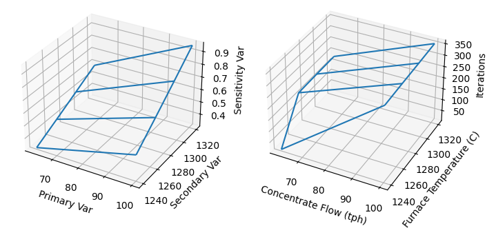
Here is the Sensitivity Analysis example done with python
import syscadif
import numpy as np
import matplotlib.pyplot as plt


sc = syscadif.SysCADCom()
ScdPrj = r'C:\SysCAD139\Examples\65 Smelting\Copper Flash Furnace Example.spf\Project.spj'
sc.OpenProject(ScdPrj)  ## Open project

VarTags = {"Cu_Concentrate.QmReqd (t/h)": (62, 100, 2),
           "Controllers.Cfg.[2].Spt":     (1240, 1320, 4),
           ## add further variables as needed Tagstr: (vmin, vmax, npts)
           }
SensTags = ["P_005.Qm (t/h)", "$Solver.Convergence.Iterations"]

V  = tuple(np.linspace(*v) for v in VarTags.values())
mgrid  = np.meshgrid(*V)

@np.vectorize
def f(*U):
    '''Funtion to set primary variables, run SysCAD, and return sensitivity variable'''
    for u, t in zip(U, VarTags.keys()):
        sc[t] = u
    sc.run()
    return tuple(sc[t] for t in SensTags)

## Now evaluate the SysCAD model over a n-dimensional grid (n is the number of VarTags)
## This returns a tuple of n-dimensional arrays, each being the values of the sensitivity variables at the gridpoints defined by meshgrid.
Z = f(*mgrid)

X, Y = mgrid
fig = plt.figure()
ax = fig.add_subplot(1,2,1, projection='3d')
ax.plot_wireframe(X, Y, Z[0])
ax.set_xlabel("Primary Var")
ax.set_ylabel("Secondary Var")
ax.set_zlabel("Sensitivity Var")
ax = fig.add_subplot(1,2,2, projection='3d')
ax.plot_wireframe(X, Y, Z[1])
ax.set_xlabel("Concentrate Flow (tph)")
ax.set_ylabel("Furnace Temperature (C)")
ax.set_zlabel("Iterations")

plt.show()
sc.Close()
We could run this as a set of scenarios, but for fun we use a numpy meshgrid to create the points at which we want to evaluate the model. We also create a vectorized function which is used to evaluate the model at each of the points. We use the resulting 2D array to plot a 3D graphic.
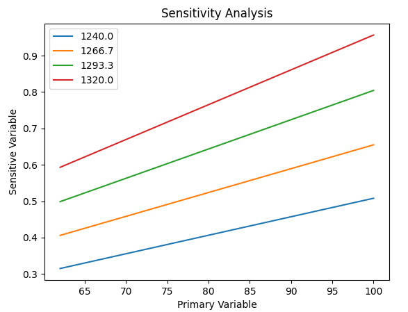
Even easier if we just want to create a 2D plot like the original example
for Y, v in zip(Z[0], V[1]):
    plt.plot(V[0], Y, label = ("%6.1f" % v))
plt.legend()
plt.title("Sensitivity Analysis")
plt.ylabel("Sensitive Variable")
plt.xlabel("Primary Variable")
This example can easily be extended to more primary tags and sensitivity variables. Just add more items to the dictionary of primary tags (VarTags), and list of sensitivity tags. The code creates a meshgrid of the ranges, and call the vectorized function f on the meshgrid. This returns a tuple of the sensitivity variables as numpy arrays, which can be used for plotting or further analysis. This may involve a lot of evaluations of SysCAD!
If we had five primary variables, each to be evaluated at four points and returning 10 sensitivity variables, we would require [math]\displaystyle{ 4^5 = 1024 }[/math] evaluations of the flowsheet, and the vectorized function call would return 10240 data points.
Washer Example
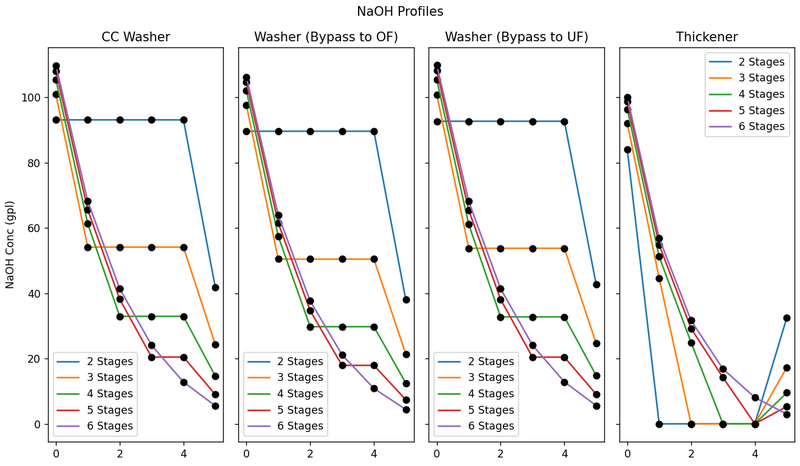
Here is the Washer Example Project showing the NaOH concentration profiles.
import numpy as np
import matplotlib.pyplot as plt

import sys
sys.path.append(r"C:\SysCAD139\BaseFilesUser\Scripts")   ## syscadif.py is saved in a subdirectory of BaseFilesUser
import syscadif

scprj = r"C:\SysCAD139\Examples\03 UnitModels\Counter Current Washer Example.spf\Project.spj"

WashTags  = ["CCW_CONTROL.CCW{}_Online",
             "WASHER_CONTROL.CCD00{}_Online",
             "WASHER_CONTROL.CCD10{}_Online",
             "TH_CONTROL.TH{}_Online"]
OutTags = ["CCW_CONTROL.UF{}_NaOHConc (g/L)",
           "WASHER_CONTROL.UF00{}_NaOHConc (g/L)",
           "WASHER_CONTROL.UF10{}_NaOHConc (g/L)",
           "TH_CONTROL.UF{}_NaOHConc (g/L)"]

def setStages(ion):
    '''Set all the on/off states for washers'''
    for i in range(2, 7):
        for tg in WashTags:
            sc[tg.format(i)] = (i<ion)

def getData():
    return np.array([sc[tg.format(i)] for tg in OutTags for i in range(1, 7)])

def t0():
    plt.ion()
    fig, axs = plt.subplots(1, 4, sharey=True, tight_layout=True)

    for i in range(2, 7):
        setStages(i)
        sc.run()
        dd = getData().reshape((4, 6))
        for ax, dat in zip(axs, dd):
            ax.plot(dat, label=f"{i} Stages")
            ax.plot(dat, "ko")
    for ax in axs: ax.legend()
    for ax, ss in zip(axs, ["CC Washer", "Washer (Bypass to OF)", "Washer (Bypass to UF)", "Thickener"]):
        ax.set_title(ss)
    axs[0].set_ylabel("NaOH Conc (gpl)")
    plt.suptitle("NaOH Profiles")
    plt.savefig("fig4.png")
    plt.show()

sc = syscadif.SysCADCom()
sc.OpenProject(scprj)
sc.run()

t0()

sc.CloseProject()
sc.Close()
|
More 3D plots
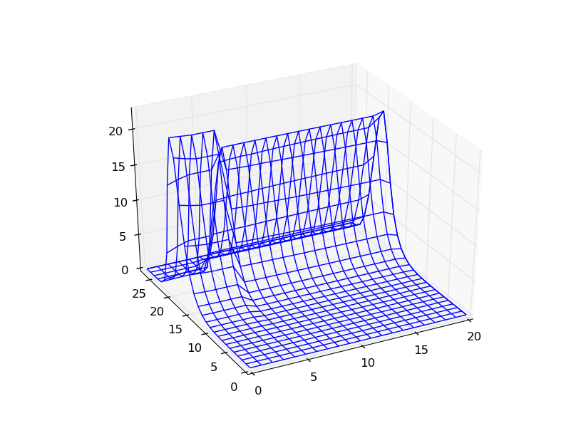
This example pulls particle size distributions data for a series of pipes in the Distributed Precipitation and Classification Example without ever running SysCAD. It then makes a 3d plot showing the variation in PSD curve along the tank row.
import syscadif  ## SysCAD COM interface class
import numpy as np
import matplotlib.pyplot as plt


sc = syscadif.SysCADCom()
ScdDir = r'C:\SysCAD%d' % sc.build
ScdPrj = r'\Examples\10 Alumina\PSD Precipitation & Classification Example.spf\Project.spj'

sc.OpenProject(ScdDir+ScdPrj)  ## Open project
pipelist = ["P_115_", "P_116_"]+["P_0%02d" % i for i in range(4, 24, 2)]+["P_121"]
sizetags = [".Qo.Sz.I%d.FP.Al[OH]3(s) (%%)" % i for i in range(28)]
fig = plt.figure()
ax = fig.add_subplot(111, projection='3d')
X, Y = np.meshgrid(np.arange(len(pipelist)),
                  np.arange(len(sizetags)))
Z = np.array([ [sc[pipe+s] for pipe in pipelist] for s in sizetags])
ax.plot_wireframe(X, Y, Z)
plt.show()
