Discussion: Annual Climate Data for Dynamic Modelling, Part III
Navigation: Product Blog ➔ Discussion Pages ➔ Annual Climate Data for Dynamic Modelling, Part III
| Part I | Part II | Part III |
|---|
Related Links: Waveform Controller, Dynamic Evaporation Ponds
Recap
In the previous discussion page we looked at a PGM implementation of an averaging periodic spline for smooth input of average annual climate data (e.g. rainfall and evaporation rates). In this discussion, we will look at the implementation in the updated Waveform Controller.
New Waveform Controller Options
SysCAD already had a Waveform Controller which was intended for simple periodic waveforms like sine waves and sawtooth models. Since annual climate data is also periodic, it makes sense to extend the waveform controller to handle general periodic data.
In this discussion page we demonstrate the use of the updated waveform controller to provide smoothed environmental data to models. We will use the rainfall data from the Profile Controller wiki page to demonstrate the features of the new model.
Using the New Controller Options
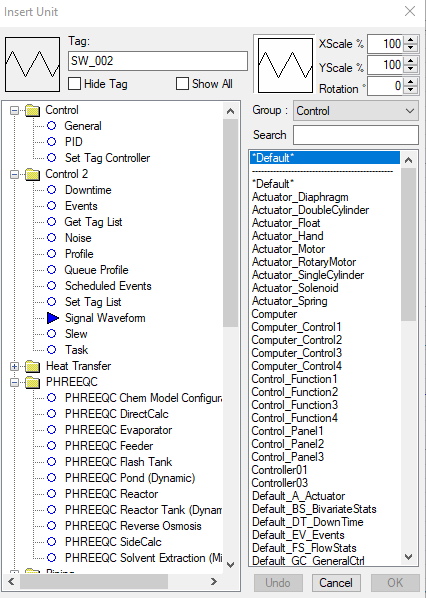
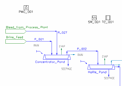
The Signal Waveform controller is inserted like any other controller model (e.g. SW_001). You may need to edit the configuration file if the Dynamic Control models are not included.
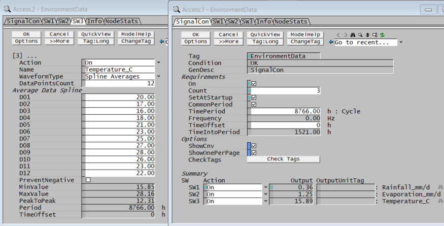
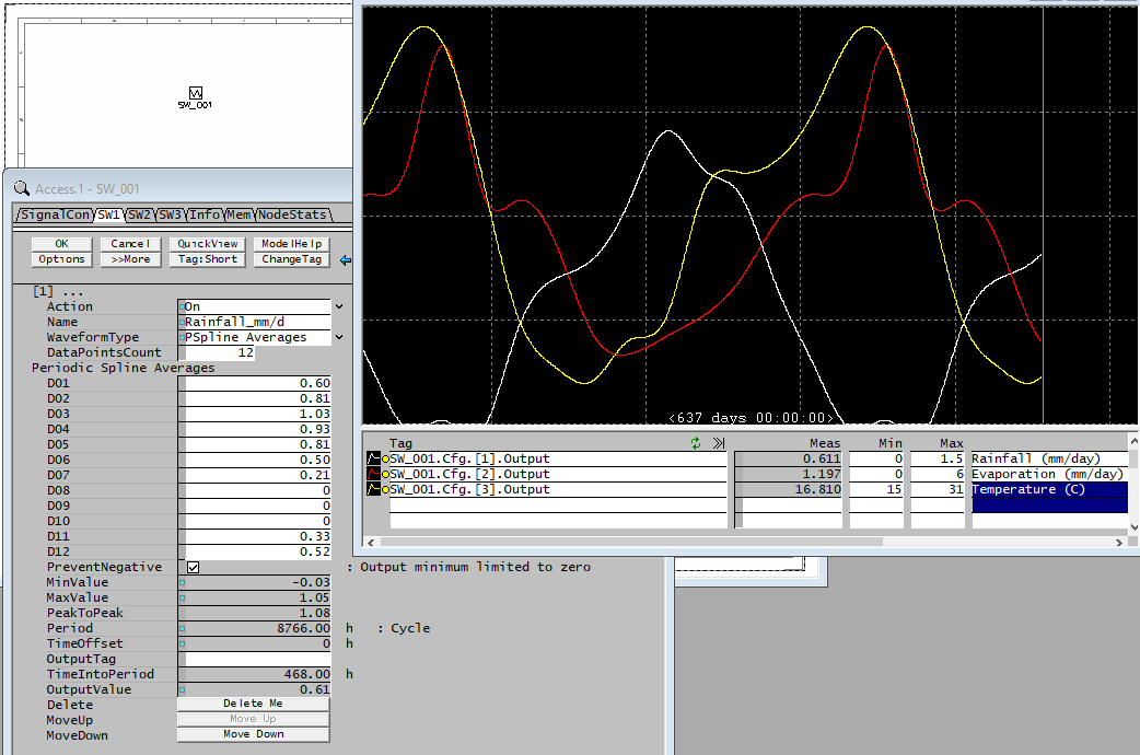
As in Part II, we will want output signals for Rainfall, Evaporation and Ambient Temperature. The waveform controller can have multiple models so all of these can be done within a single controller unit. Each of the outputs has a common period (one year) so we can select the CommonPeriod option on the first tab. Data for each of the signals is then entered into the appropriate tab with a DataPointsCount of 12.
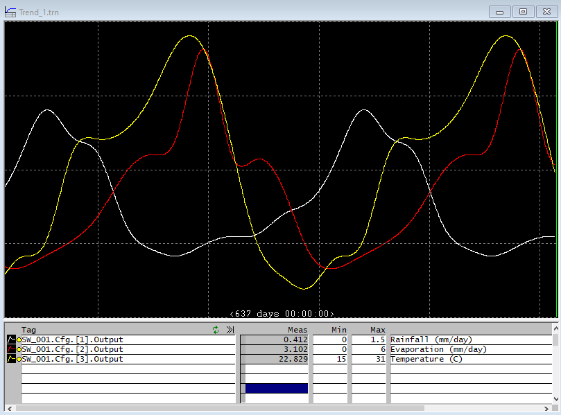
We now get smooth signals for the environmental data, which we can use as inputs to our Dynamic model!
The Julian Year
You may have noticed that SysCAD doesn't include Months or Years as time units. This is because there is some ambiguity in the length of a year, and even more in the length of a month.
For purposes of Dynamic modelling we define the year as the Julian year, which is exactly 365.25 days long (or 8766 hours). So in running a Dynamic model there will be a slight mismatch between the true calendar date (based on the Gregorian year) and the year defined by a fixed period. The Gregorian year is based on skipping leap years at the turn of the centuries three times every 400 years, so that Y2K (2000) was actually a leap year, while 1800, 1900 and 2100 are not. The difference between the Gregorian year and the Julian year is 0.18 hours or just over ten minutes. Running a Dynamic model for a century will result in a 'mismatch' between the "true" Gregorian calendar time and the Julian calendar time of less than a day, so this is not likely to significantly affect the results of the model. Plus, rainfall and temperatures a century in the future are likely to be significantly different due to climate change, so it is unlikely you will want to run an environmental model this far into the future!
Of course this Waveform controller can also be used for period data over much shorter timespans, but it is worth considering the implications of "inconsistent periodicity".
Time Control in Dynamic Simulation
There are some subtle issues in the timebase used by SysCAD in a Dynamic model and these may affect how the model should be initialized and run. One approach is to ensure that the time is reset each time the model runs; however with the SOP pond model we may want to run for a period of time and save it, then experiment with different control strategies from that point onwards.
Part of this relates to the Historian which is how SysCAD saves data for the Trend Window. If you save a model at a particular point in time with Historian data, then reopen and rerun it, the Historian Time will advance, so that reverting to the saved model will end up at a different time in the annual cycle. If a pond model saved in the middle of winter is reopened with the time now in midsummer, the temperature is higher, so the pond conditions have a large step change (so control on volume is likely to see a large step change). We currently working on modifying SysCAD to allow better control of the timebase in Dynamic models but be aware that care is needed here.
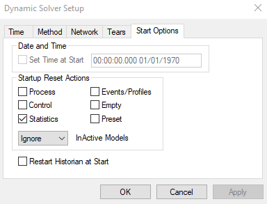
To allow the model to restart at the same time as the end of the last run, disable the reset of Events/Profiles in the Dynamic Solver Setup Dialog.
Using the Output Periodic Data
The waveform controller allows you to specify an OutputTag, but here we want to apply the rainfall and temperature to a number of pond models, so we can leave this field blank. We then use a Set Tag Controller to copy the rainfall and temperature data to each of the pond models.
Nonnegative Values
One situation where these models might have problems is when they could predict negative values for rainfall or evaporation. During a long dry spell, there may be no rain at all, and fitting a smooth curve through this would end up with negative rainfall in places:
There is a checkbox option PreventNegative which can be used to ensure the output is physically meaningful. As the true spline is no longer applied, this will cause a minor discrepancy vs the original data (e.g. giving a small positive value over periods where the average value is actually zero) because of the algorithm behind the spline fit. We are working to fix this in a future release.
Waveform Controller Methods
Described in detail on the Waveform Controller wiki page, there are various other configurations and options for customising the signal output:
- Linear DataPoints uses a linear interpolation between the data points. (Equivalent to using a Profile controller with Linear on.)
- Linear Averages uses the input data as average values for each time interval. (Equivalent to using a Profile controller with Linear off.)
- Spline DataPoints is a regular cubic spline fit through the specified data points.
- Spline Averages is a regular cubic spline fit to calculated points such that the area under the curve in each interval is the same as for Linear Averages.
- BSpline DataPoints is a cubic B-spline (basis spline) through the data points (similar to Spline DataPoints, but different mathematics to generate the curve).
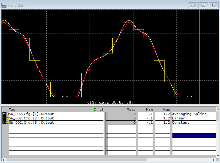
The example below shows Linear DataPoints (red), Linear Averages (yellow) and Spline Averages (white):
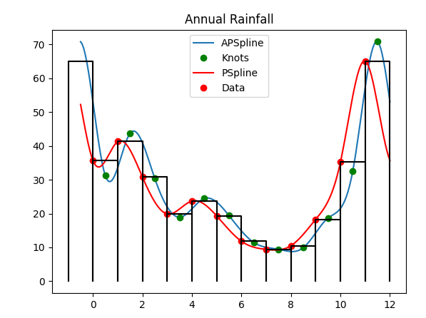
The distinction between a regular periodic spline (Spline DataPoints) and the averaging periodic spline (Spline Averages) is explained with the diagram below. Use a regular spline if the curve is to pass through the supplied data points. Use an averaging spline if the data input represents the average over the interval. Note that there is also an option UseAsMidpoints to shift the regular spine by half an interval such that the curve to passes through the midpoint of the intervals (this is always done for the averaging case).
Note here that both curves use the same data input (red points). The regular case uses these directly as spline knots, while the averaging case calculates new knots (green points) such that area under the curve is conserved.
First Posted: 25 May 2022
Reference Build: 139.30918
For questions or feedback, please contact us at [email protected].
