Size Distribution Definition
Navigation: Models ➔ Qualities Models ➔ Size Distribution (PSD) ➔ Size Distribution Definition
Related Links: Size Distribution (PSD), Size Configuration, Size Distribution Models
Introduction
You can create a size distribution on the following units:
- A Feeder-Cross Page Connector unit; and
- A pipe on the Qi tab page.
See the Qualities for details on the steps required to create the distribution.
Once a Size distribution has been created the Define size tab page (DSz) will be activated. This allows the user to define the Size Distribution, or Distributions if more than one solid species has been specified, for the solids in the unit. There are a number of different methods of defining the Size Distribution and these will be described below.
Method
The user may then define the Size Distribution using a number of different methods:
- Rosin-Rammler
- Modified Rosin-Rammler
- Gaudin-Schuhmann
- Lynch
- Linear Interpolate
- Data Points: Interval Fraction
Each of these methods will be described in the following sections, together with the data fields in the Access window.
Single Definition
In addition to this, the user may wish to initially set all solids to have the same Size Distribution, even if they may be specified individually. If the SingleDefn tick box is enabled, then the user may set a single definition for multiple size distributions.
This can be really useful, as often a user has a single size distribution for the feed to the plant, but then the different solids will be crushed or milled differently.
- In the configuration file individual solids are set up to have their own size distributions.
- In the Feeder to the plant, tick the 'SingleDefn' tick box and enter a single size definition, using any of the methods described below.
- In the Crush and Mill units, set each solid species to have individual product size distributions.
Rosin-Rammler
In this and all subsequent definitions [math]\displaystyle{ d_i }[/math] is the top size of interval [math]\displaystyle{ i }[/math], that is the interval containing particles with diameter [math]\displaystyle{ d_{i-1} \lt d \lt d_i }[/math]
The Rosin-Rammler equation used to determine the size distribution is as follows:
- [math]\displaystyle{ W_p=100 \times \left(1- \exp \left( \; - \left( {d_i}/{a} \right)^{b} \; \right) \right) }[/math]
where:
[math]\displaystyle{ W_p }[/math] = mass fraction passing (%) [math]\displaystyle{ a }[/math] = size at which (100/e) = 36.8% of particles retained [math]\displaystyle{ b }[/math] = constant = slope of the plot of [math]\displaystyle{ \ln(100/W_p) }[/math] vs [math]\displaystyle{ \ln x }[/math]
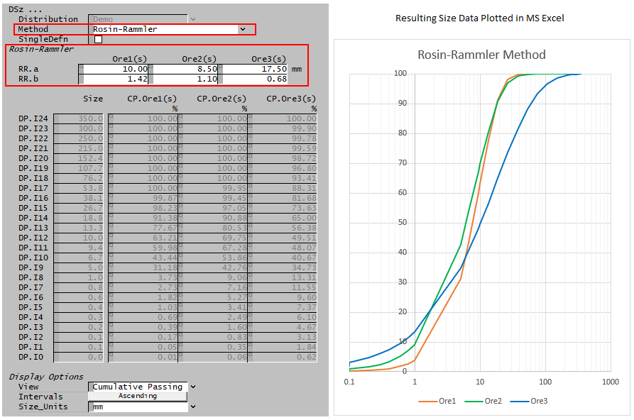
An example of the Access window using Rosin-Rammler is shown below:
In this case, the user sets the Rosin-Rammler values of 'a' and 'b' for each solids set and SysCAD then calculates the mass fraction retained for each size interval.
Modified Rosin-Rammler
The modified Rosin-Rammler equation used to determine the size distribution is as follows:
- [math]\displaystyle{ W_p=100\times\left\{1-\exp \left[ -0.693147 \; \left(d_i/d_{50}\right) ^{m} \; \right]\right\} }[/math]
where:
[math]\displaystyle{ W_p }[/math] = mass passing (%) [math]\displaystyle{ d_{50} }[/math] = size at which 50% of particles retained by mass [math]\displaystyle{ m }[/math] = sharpness constant
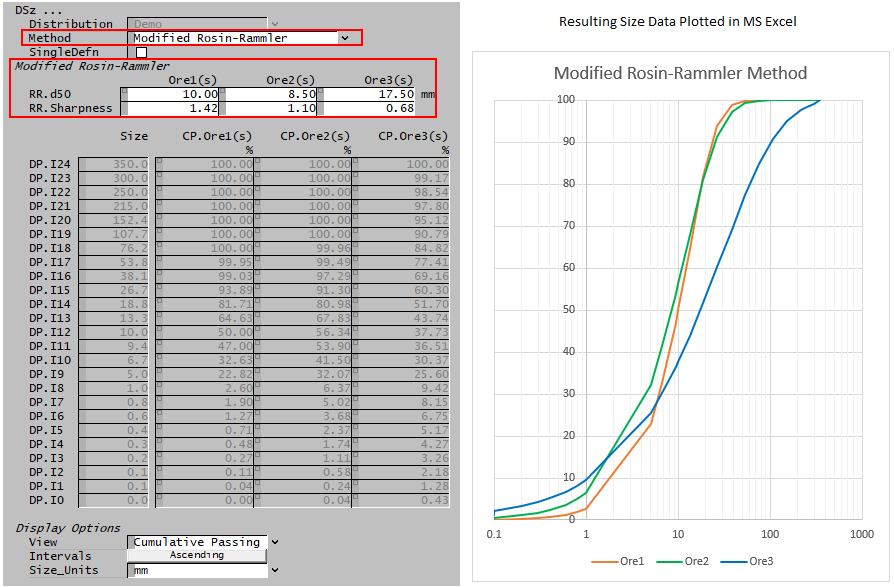
An example of the Feeder Access window using the modified Rosin-Rammler is shown below:
In this case, the user sets the modified Rosin-Rammler values of 'd50' and 'Sharpness' for each solids set and SysCAD then calculates the mass fraction retained for each size interval.
Gaudin-Schuhmann
The Gaudin-Schuhmann equation used to determine the size distribution is as follows:
- [math]\displaystyle{ W_p=100\times\left(\cfrac{d_i}{k}\right)^{m} }[/math]
where:
Wp = mass passing (%) k = size modulus - size when Wp = 100 m = distribution modulus = slope of the log-log plot Wp vs x
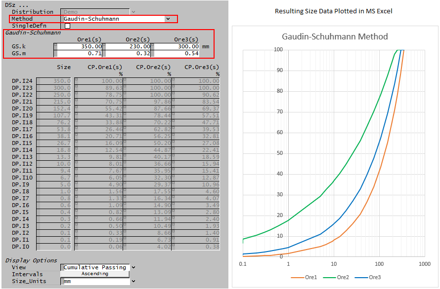
An example of the Access window using Gaudin-Schumann is shown below:
In this case, the user sets the Gaudin-Schuhmann values of 'k' and 'm' for each solids set and SysCAD then calculates the mass fraction retained for each size interval.
Lynch
The Lynch equation used to determine the size distribution is as follows:
- [math]\displaystyle{ W_r=100\times\cfrac{\exp(\alpha)-1}{\exp\left(\alpha d_i/d_{50}\right)+\exp(\alpha)-2} }[/math]
where:
[math]\displaystyle{ W_r }[/math] = mass fraction retained (%) [math]\displaystyle{ d_{50} }[/math] = size at which 50% of particles retained by mass [math]\displaystyle{ \alpha }[/math] = [math]\displaystyle{ 1.54 m - 0.47 }[/math] [math]\displaystyle{ m }[/math] = sharpness constant
- Note that this defines the fraction retained so that when [math]\displaystyle{ d_i }[/math] is large, [math]\displaystyle{ W_r = 0 }[/math] The fraction passing [math]\displaystyle{ W_p = 1-W_r }[/math]
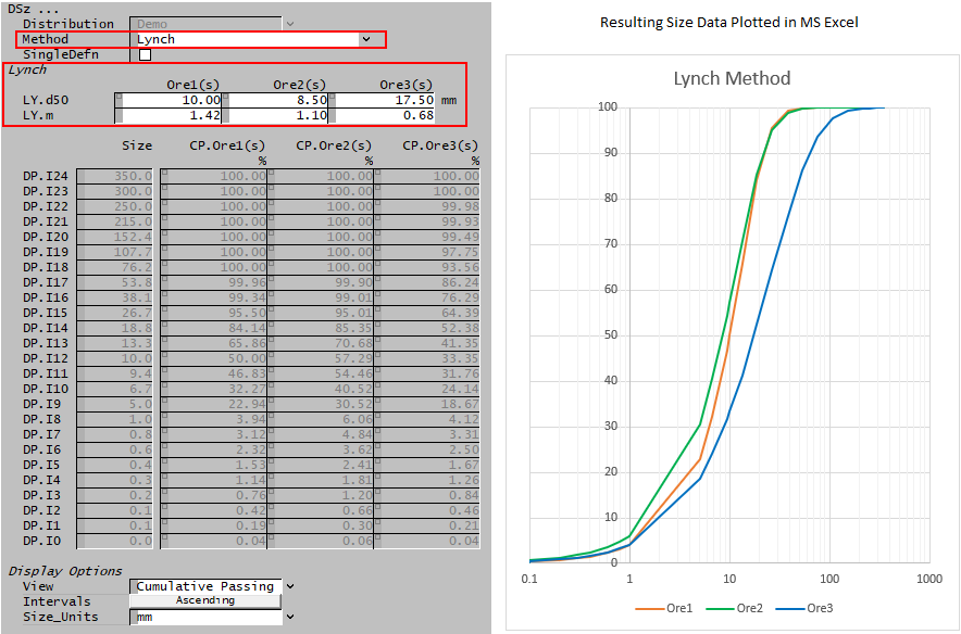
An example of the Feeder Access window using the Lynch equation is shown below:
In this case, the user sets the Lynch values of 'd50' and 'm' (sharpness) for each solids set and SysCAD then calculates the mass fraction retained for each size interval.
Linear Interpolate
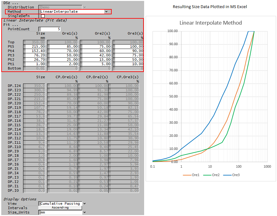
This method takes a user defined number of data points (up to a maximum of 50) and interpolates to determine the size distribution across the full range of size intervals. Linear interpolation is performed using particle size on a log scale.
The Access window below shows the Linear Interpolation method.
- Here we have chosen to define 5 points for each solid size distribution.
- We have chosen sizes that match the existing size data points for ease of checking, however, these values can be any size within the given size distribution - in the example below any value between 0.01 and 350mm.
- The user then enters the fraction passing at the selected points.
In this case, the user sets the required number of points, and the values at the size intervals for each solids set and SysCAD then calculates the mass fraction for each size interval.
If user needs to input data with many data points, can use a PGM file to load in the data (saved in a csv file) at the start of the project. Please see Set A Table of Values Using Matrix Class for an example of how to do this.
Data Points: Interval Fraction
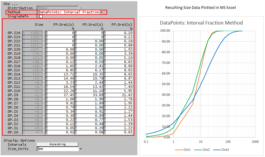
With this method the user defines the mass fraction in each individual size interval.
Note: The mass fractions across all size intervals must sum to 100%. If the user enters values such that the sum > 100% or the sum < 100%, SysCAD will adjust the mass fractions in the largest size intervals.
The Access window below shows the Data Points: Interval Fraction method:
Data Sections
The variable names that are common to all methods are described in detail in the following table. The individual methods are described in the above sections.
| Tag (Long/Short) | Input / Calc | Description/Calculated Variables / Options |
| Inputs | ||
| Distribution | Input / Display | If more than one Size Distribution has been defined for the project, then the user may select the required Size distribution in this field. If only a single Size Distribution is defined for the project, then this field displays the Size distribution. |
| Method | Rosin-Rammler | Mass fraction retained in each size interval is calculated using the Rosin-Rammler equation with two user-specified constants: a & b. |
| Modified Rosin-Rammler | Mass fraction retained in each size interval is calculated using the Modified Rosin-Rammler equation with two user-specified constants: d50 and sharpness constant. | |
| Gaudin-Schuhmann | Mass fraction retained in each size interval is calculated using the Gaudin-Schuhmann equation with two user-specified constants: k & m. | |
| Lynch | Mass fraction retained in each size interval is calculated using the Lynch equation with two user-specified constants: d50 & m. | |
| LinearInterpolate | This method takes a user defined number of data points and interpolates to determine the size distribution across the full range of size intervals. | |
| DataPoints: Interval Fraction | With this method the user directly sets the mass fraction in each individual size interval. | |
| SingleDefn | Tick Box | This is enabled when you are tracking size data independently for multiple solids species. When enabled the user can select this to set a single size distribution definition that applies to ALL solid species (rather then separate parameters for each solid). |
| The required inputs will depend on the Method chosen. The Size Distribution fields will either be display fields, or in the case of Data Entry they will be input fields. Please see Size Distribution Definition for the equations and description of these fields. | ||
| Display Options | ||
| View (Not visible for Data Entry methods) |
Interval Fraction | The table will display the calculated mass fraction in each interval fraction. |
| Cumulative Passing | The table will display the cumulative mass passing through each sieve size. In this case the top size will always display 100%. | |
| Cumulative Retained | The table will display the cumulative mass retained on each sieve size. In this case the top size will always display 0%. | |
| Intervals | Clicking on this button will toggle between displaying the size intervals in Ascending or Descending order. | |
| Size_Units | List | The user may select the display units, i.e. mm, um, etc., from a drop-down list. |
