Discussion: Annual Climate Data for Dynamic Modelling, Part II
Navigation: Product Blog ➔ Discussion Pages ➔ Annual Climate Data for Dynamic Modelling, Part II
| Part I | Part II | Part III |
|---|
Related Links: PGM, Waveform Controller, Dynamic Evaporation Ponds
Recap
In the last page we looked at the issues around generating smooth profiles for annual climate data. We will now look implementing this using some of the advanced capabilities of PGM in a General Controller. The PGM language has built-in functionality for manipulating arrays and linear/matrix algebra, and in many cases this can simplify coding of complex models. The built-in methods are also coded at low level in C++, so will be much faster than implementing the same calculations via the PGM language. (Another application of the array methods is manipulating size distribution data, and we will examine an example of this in a future discussion page.)
Theory
Splines
A regular [spline] is a curve defined piecewise by polynomials that has continuous curvature. In the simplest case, each piecewise segment is a cubic polynomial, and the curvatures are linear over each interval, matching at the knots [math]\displaystyle{ x_i }[/math]. So over the interval [math]\displaystyle{ [x_i, x_{i+1}] }[/math] the curvature is:
- [math]\displaystyle{ a_i(x_{i+1}-x) + a_{i+1}(x-x_i) }[/math]
We will assume the knots are equally spaced and the interval is 1 (so that [math]\displaystyle{ x_{i+1}-x_i = 1 }[/math]). If the values at the knots are [math]\displaystyle{ f_i }[/math] we can integrate to find the representation:
- [math]\displaystyle{ S_i(x) =\frac16 \left[a_i(x_{i+1}-x)^3 + a_{i+1}(x-x_i)^3\right] + (f_i-a_i/6)(x_{i+1}-x) + (f_{i+1}-a_{i+1}/6)(x-x_i) }[/math]
The continuity condition [math]\displaystyle{ S_{i-1}'(1)= S_i'(0) }[/math] gives the condition:
- [math]\displaystyle{ a_{i-1}+ 4a_i+ a_{i+1} = 6(f_{i-1}-2f_i+ f_{i+1}) }[/math]
If there are [math]\displaystyle{ N }[/math] data points, we have [math]\displaystyle{ N-2 }[/math] conditions (at each interior knot) and we can write these in matrix form:
- [math]\displaystyle{ \begin{bmatrix} 4 &1 &0 \cdots &0\\ 1 &4 &1 \cdots &0\\ 0 &1 &4 \cdots &0\\ &\cdots\\ 0 &0 &0 \cdots &4\\ \end{bmatrix} \begin{bmatrix} a_1 \\ a_2 \\ a_2 \\ \cdots\\ a_{N-2}\\ \end{bmatrix} = 6 \begin{bmatrix} 1 &-2 &1 &0\cdots &0\\ 0 &1 &-2 &1\cdots &0\\ 0 &0 &1 &-2\cdots &0\\ &\cdots\\ &&&\cdots &-2\quad 1\\ \end{bmatrix} \begin{bmatrix} f_0 \\ f_1 \\ f_2 \\ \cdots\\ f_{N-1}\\ \end{bmatrix} }[/math]
For a regular spline over a fixed interval we need to specify the curvature in some way at the two endpoints. The approach here is a natural spline where the curvature is defined to be zero. In any case, the system of equations is tridiagonal and can be solved efficiently. The right-hand side is actually just a column vector that can be calculated directly, but we write it in this form for reasons that will be clear soon...
Periodic Splines
For repeating (e.g. annual) data, we are actually interested in periodic splines which "wrap around" at the endpoints. Here things become more interesting! The system of equations now becomes:
- [math]\displaystyle{ \begin{bmatrix} 4 &1 &0 \cdots &1\\ 1 &4 &1 \cdots &0\\ 0 &1 &4 \cdots &0\\ &\cdots\\ 1 &0 &0 \cdots &4\\ \end{bmatrix} \begin{bmatrix} a_0 \\ a_1 \\ a_2 \\ \cdots\\ a_{N-1}\\ \end{bmatrix} = 6 \begin{bmatrix} -2 &1 &0 \cdots &1\\ 1 &-2 &1 \cdots &0\\ 0 &1 &-2 \cdots &0\\ \cdots\\ 1 &0 &0 \cdots &-2\\ \end{bmatrix} \begin{bmatrix} f_0 \\ f_1 \\ f_2 \\ \cdots\\ f_{N-1}\\ \end{bmatrix} }[/math]
The left-hand size matrix is no longer tridiagonal because of the non-zero elements in the corners. However, it does have other interesting properties that make it amenable to direct analysis - in particular it is circulant so that each row (and column) consists of the same elements shifted to the right (or down) and wrapping around at the edges, and there is a whole lot of interesting theory and application for such matrices.
Of particular interest here, the inverse of a circulant matrix is also circulant, as are the sums and products of two circulant matrices. So we can represent a circulant matrix by just a vector. In that case, the product of two circulant matrices is represented by the circular convolution of the vector representations. And the product of a circulant matrix with a column vector is just the circular convolution of the vectors. (As we mentioned in Part I, we added new array operations CircConv and CopyCircConv to the PGM array class for just this reason!)
Rather than writing out this in full we write [math]\displaystyle{ \mathbf{A a} = \mathbf{B f} }[/math] where the boldface capital is a matrix and the boldface lower case is a column vector. We can write the solution to this equation as [math]\displaystyle{ \mathbf{a} = \mathbf{A^{-1} B f} }[/math]. If we precompute [math]\displaystyle{ \mathbf{A}^{-1} \mathbf{B} }[/math] for any particular value of N, then we have a direct calculation of the curvatures.
Averaging Splines
As we described in the previous discussion page, we are looking for a spline for which the area under the curve in each interval is equal to the input data, which we will write as [math]\displaystyle{ \bar f_i }[/math] (e.g. monthly rainfall data over a year). In this case we no longer know the values at the knots [math]\displaystyle{ \mathbf f }[/math]. It is convenient to locate the knots at the midpoints of the intervals, and integrate the form for [math]\displaystyle{ S_i(x) }[/math]:
- [math]\displaystyle{ \frac18 \begin{bmatrix} 6 &1 &0 \cdots &1\\ 1 &6 &1 \cdots &0\\ 0 &1 &6 \cdots &0\\ \cdots\\ 1 &0 &0 \cdots &6\\ \end{bmatrix} \begin{bmatrix} f_0 \\ f_1 \\ f_2 \\ \cdots\\ f_{N-1}\\ \end{bmatrix} -\frac1{384} \begin{bmatrix} 18 &7 &0 \cdots &7\\ 7 &18 &7 \cdots &0\\ 0 &7 &18 \cdots &0\\ \cdots\\ 7 &0 &0 \cdots &18\\ \end{bmatrix} \begin{bmatrix} a_0 \\ a_1 \\ a_2 \\ \cdots\\ a_{N-1}\\ \end{bmatrix} = \begin{bmatrix} \bar f_0 \\ \bar f_1 \\ \bar f_2 \\ \cdots\\ \bar f_{N-1}\\ \end{bmatrix} }[/math]
We write this as [math]\displaystyle{ \mathbf{C f} - \mathbf{D a} = \mathbf{\bar f} }[/math]
So now, instead of solving for the curvatures [math]\displaystyle{ \mathbf{a} }[/math] directly, we have two systems of equations - we need to determine the knot values [math]\displaystyle{ \mathbf{f} }[/math] first, and then find the curvatures. We can use the solution we already have and we find:
- [math]\displaystyle{ \mathbf{f} = \left[\mathbf{C} - \mathbf{D} \mathbf{A}^{-1}\mathbf{B}\right]^{-1} \mathbf{\bar{f}} }[/math]
Again, for any particular value of N we can precompute the array [math]\displaystyle{ \mathbf{R} = \left[\mathbf{C} - \mathbf{D} \mathbf{A}^{-1}\mathbf{B}\right]^{-1} }[/math].
That's enough theory for the time being, so now let's look at implementing this in PGM.
Implementing the PGM Code
Array Precalculation
First we need to precalculate the arrays. We could do this in PGM if we really need to implement a general case with user-specified number of data points, but since we are dealing with a fixed number of data points (average monthly data, so 12) we can cheat and pre-calculate these externally. In this case we'll use numpy (numerical Python).
import numpy as np
import numpy.linalg as la
## the eye function returns a 2D array with ones on the specified diagonal and zeros elsewhere
def mgen(i, d, do):
   return d*np.eye(i)+do*(np.eye(i, k=1) + np.eye(i, k=-1)+ np.eye(i, k=i-1) + np.eye(i, k=-(i-1)))

i = 12
A = mgen(i, 4, 1)
B = mgen(i, -12, 6)
C = mgen(i, 6, 1)/8
D = mgen(i, 18, 7)/384
AB = np.matmul(la.inv(A), B)
print ("AB = ", AB[0], "\n")
R = la.inv(C-np.matmul(D, AB))
print ("R = ", R[0])
This gives:
AB =  [-4.39230769  2.78461538 -0.74615385  0.2        -0.05384615  0.01538462
       -0.00769231  0.01538462 -0.05384615  0.2        -0.74615385  2.78461538]

R  =  [ 1.1998816  -0.13197293  0.04355866 -0.01571306  0.00576095 -0.00231401
        0.00147916 -0.00231401  0.00576095 -0.01571306  0.04355866 -0.13197293]
PGM Code
We are interested in annual monthly data, so N = 12. Since we want to use this for rainfall, temperatures and other data, it is a good idea to create a reusable PGM class to do the work.
; Precalculated arrays for N = 12
array AB = {-4.39230769,  2.78461538, -0.74615385,  0.2,        -0.05384615,  0.01538462,
            -0.00769231,  0.01538462, -0.05384615,  0.2,        -0.74615385,  2.78461538}
array R  = { 1.1998816,  -0.13197293,  0.04355866, -0.01571306,  0.00576095, -0.00231401,
             0.00147916, -0.00231401,  0.00576095, -0.01571306,  0.04355866, -0.13197293}

class CRainDance
   array f    ; calculated values at knots
   array a    ; calculated curvature at knots
   array data ; raw data (monthly averages) loaded from a file
   integer i0, i1
   real x0, x1, t1, a0, a1, f0, f1

   sub Init(str datafile)
      data.load(datafile)
      f.CopyCircConv(R, data) ; Convolution of data to find knot values
      a.CopyCircConv(AB, f)   ; Convolution to find curvatures
   endsub

   function Eval(real t)
      t1 = mod(t-0.5,12)
      if t1<0
         t1 = t1+12
      endif
      i0 = trunc(t1)
      i1 = mod(i0+1, 12)
      x0 = t1-i0
      x1 = 1-x0
      a0 = a.getAt(i0)
      a1 = a.getAt(i1)
      f0 = f.getAt(i0)
      f1 = f.getAt(i1)
      return (a0*x1^3 + a1*x0^3)/6+(f0-a0/6)*x1 + (f1-a1/6)*x0
   endfunct
endclass
The PGM array class load() method initializes an array with the values in the specified file, which should be in the Project folder. So to use this, we just create instances for rainfall, temperature and evaporation via the Init() subroutine on solve initialisation, and then call the Eval() function each iteration.
PageLabel("DailyData")
real Rainfall*("L", "m")<<0.4>>
real AmbientT*("T", "C")<<20>>
real Evaporation*("L", "m")<<5>>
real YearFrac@
real TNow@
CRainDance raind
CRainDance evapd
CRainDance tempd

Sub InitialiseSolution()
  raind.Init("rain.txt")
  tempd.Init("temp.txt")
  evapd.Init("evap.txt")
EndSub

;--- Logic - executed at EVERY step ---

TNow = Time()/3600
YearFrac = 12.0*mod(TNow, 8766.0)/8766.0
RainFall = raind.Eval(YearFrac)
Evaporation = evapd.Eval(YearFrac)
AmbientT = tempd.Eval(YearFrac)

["Evap_Pond_Control.Rain (m)"] = RainFall
["Evap_Pond_Control.Evap (m)"] = Evaporation
["Evap_Pond_Control.PondTemperature (C)"]= AmbientT
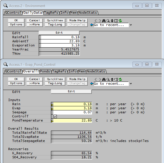
The values are sent to the main pond control PGM (Evap_Pond_Control) and away we go...
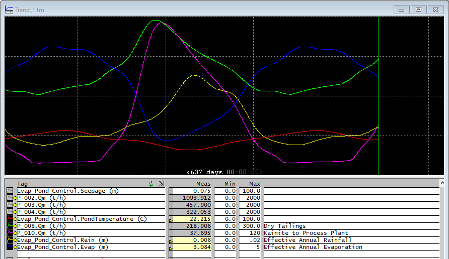
The results are smooth curves for rainfall, temperature and evaporation. And the model runs stably!
Copying the Data Files
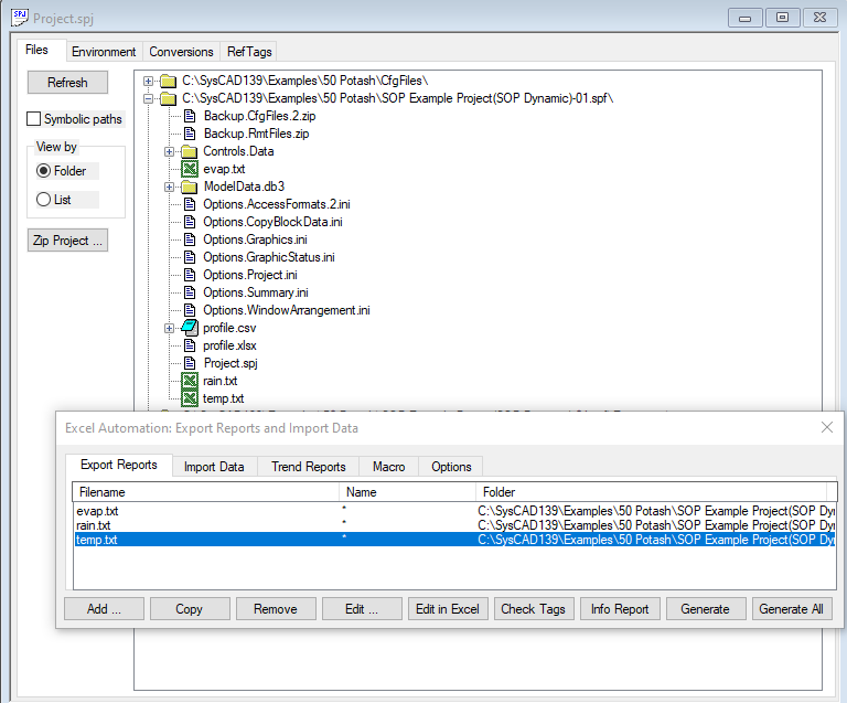
Since we are reading the monthly data from text files, we need to be sure these are also copied whenever we save a new copy of the project. Normally this would be done by manually copying the files across. We could also store the files outside of the project folder and supply a hard-coded path to the location.
Alternatively, we could use a sneaky trick to copy specific files when you create a new version of a project. We add the files as Excel reports via Add... Browse... In Save As Type choose Select All Files (*.*) and select the text files. This will add the files to the project's included file list.
New Waveform Controller Options
Since this functionality is very useful we have added it to the Waveform Controller model - so you don't need to use PGM at all. That said, using classes and array methods lets you do lots of things with PGM that you can't do with the standard SysCAD models, so it is good to be familiar with these techniques.
In the next discussion page we will look at using the new functionality of the Waveform controller.
First Posted: 24 May 2022
Reference Build: 139.30918
For questions or feedback, please contact us at [email protected].


