Discussion: Annual Climate Data for Dynamic Modelling
Navigation: Product Blog ➔ Discussion Pages ➔ Annual Climate Data for Dynamic Modelling
| Part I | Part II | Part III |
|---|
Related Links: Profile Controller, Waveform Controller, Dynamic Evaporation Ponds
Overview
In a Steady State model of Evaporation Ponds, the annual rainfall, temperature and evaporation rates are key parameters, fixed at a constant average value for the applicable period. For a corresponding Dynamic Model we would instead typically have monthly data input via a Profile Controller to modify the values as the model is solving.
For any Dynamic model stability is always a concern. The discontinuous values set by a profile controller at the beginning of each month can be especially problematic. We illustrate this with a Dynamic version of the Sulphate of Potash (SOP) Example Project and discuss some approaches for turning the profile data into smooth input.
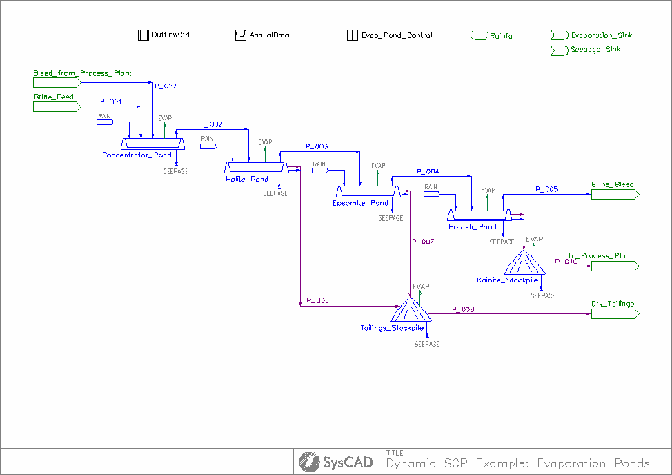
Dynamic SOP Project
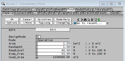
We can convert the SOP project to Dynamic by simply creating a Dynamic version of the configuration file (SOP Example_Dyn.cfg) including Dynamic controllers, and open the project with the Alternate Configuration. There are also a few changes we need to make to the Dynamic model. First, the Dynamic Tank model now has surge capacity, so we need to specify the volume. We can do this simply by adding a MaxDepth parameter to the Pond model procedure (MP), then calculate and set the tank volume on initialization using the Area parameter which already exists. For later use, we also add a Level parameter which could be used for controlling the operating level.
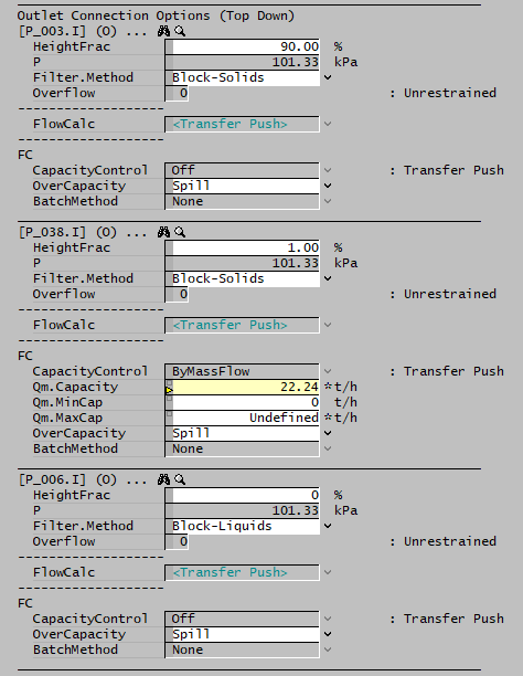
For now, we just allow the tank to fill to a pre-specified level which is determined by the height fraction of the outlet pipe, which we set to 90%. We also need additional outlets for the Halite, Epsomite and Potash ponds so we can recover solids. The dynamic tank model doesn't presently allow specification of a mixed phase composition, but we can use a Filter to block liquids and recover the solids. We need to add another outlet with Block Solids Filter where we can add the liquid that comes to the Tailings and Kainite Stockpiles and control that with a ratio controller reading the solids flow.
For the moment we don't model the process area, so we just input a fixed flow to the Bleed from Process Plant feeder. Finally, we are going to control the temperature of the ponds as well, so we enable a CEHX Evaluation block as well, for now just having a fixed temperature of 25°C.
This model just has the reactions and evaporation operating on the pond feed. A more realistic approach is to operate on the Pond contents instead using Content Reaction Blocks (CRB).
Adding Annual Data
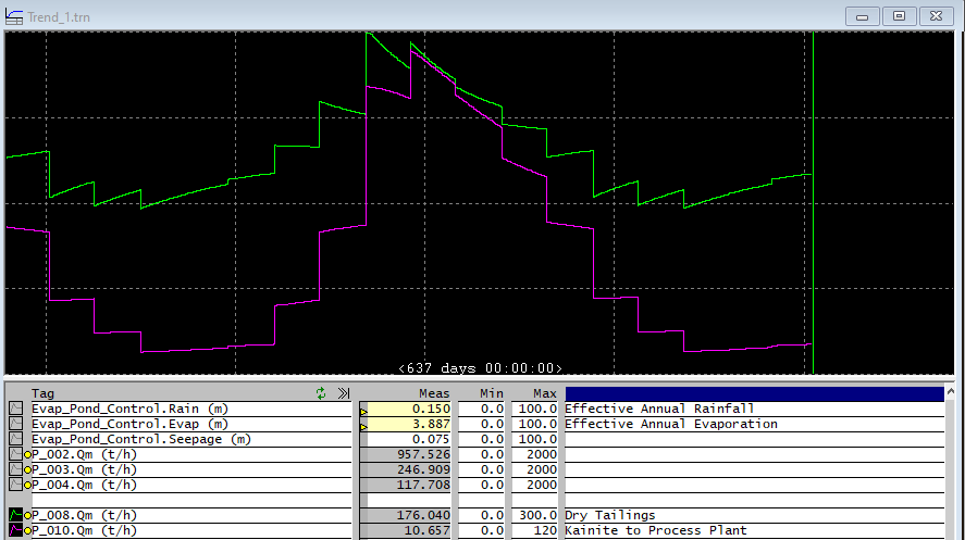
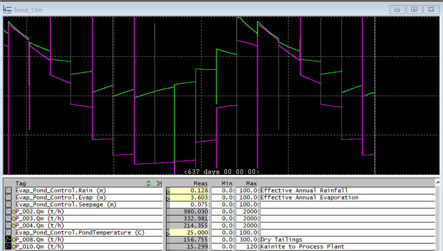
We add a Profile Controller, and use example monthly data, but with evaporation scaled to be more consistent with the 4m of annual evaporation in the Steady State model. Running this model we can see how the pond production varies over an annual cycle. There is obviously a large seasonal variation in Kainite production, so we should store this in the Kainite stockpile and remove it at a controlled rate to keep the process plant running with fairly uniform input.
The step changes that we see in the outputs due to changes in rainfall and evaporation are obviously unrealistic but the model at least runs and we can visualise roughly what is going on. However we start to get into real trouble if we add temperature control via the CEHX evaluation block. We find that the step change in temperature gives a large spike or drop in the outflow - the density is changed and so the level is suddenly increased or decreased.
This simplified model can handle these spikes in flow on subsequent iterations, but more detailed models - e.g. where we determine solids yield using accurate PHREEQC solubility calculations - become completely unstable with pond outflow varying between zero and a large value every step, rather than just at the points where we change the pond temperature.
Smoothing Data using Periodic Spline
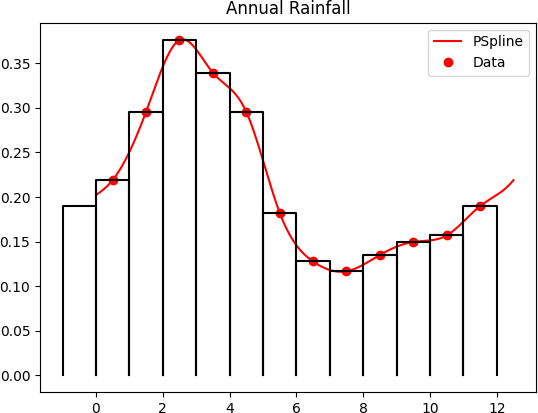
We can generate smooth output for the environmental data by using a Periodic Spline fit to the data points. A periodic spline has curvature and slope at the first point equal to that at the last point (to allow smooth repetition over multiple years).
There is however one minor issue here - if we look at the rainfall for month three, we see the monthly rainfall (represented by the area under the red curve) is less than the average rainfall for that month since the red curve lies under the black box which represents the total monthly rainfall. So directly fitting a spline to the data may underestimate or overestimate the actual monthly rainfall.
Instead, we need to find a spline fit that can accurately represent the average monthly data - such that the area under the curve over each interval is equal to the average value. A novel solution was found using circulant matrices, Fourier convolutions and Chebyshev polynomials, which was then implemented in PGM code.
Averaging Periodic Spline
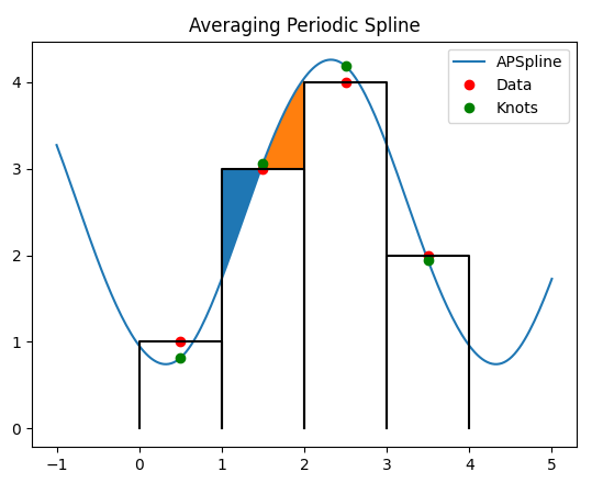
In this so-called Averaging Periodic Spline you find not only the curvatures at the knots, but the knot values as well, which are adjusted to give the correct area under the curve. In this simplified example shown here the shaded areas are equal, and thus the area under the curve is correct:
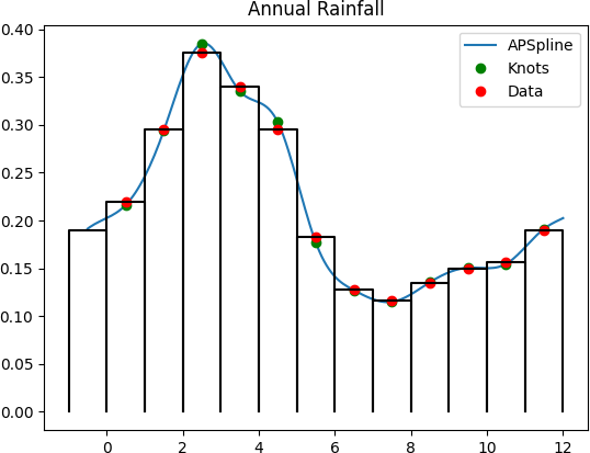
Applying this to the rainfall data we get a modified spline that ensures we are providing the correct total monthly rainfall to the model as it runs.
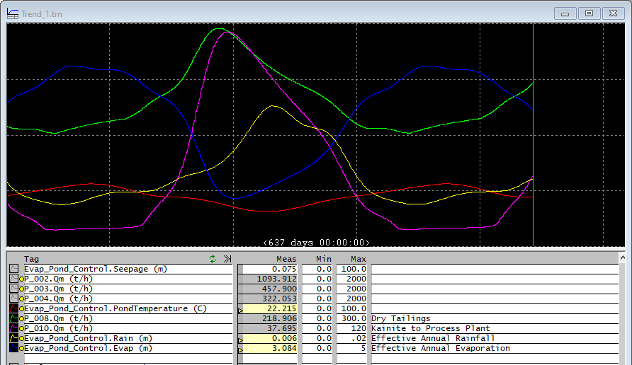
Implementing this in PGM is relatively straightforward (especially after adding a new array methods for circulant convolution, but that is another story). The results are gratifyingly stable and realistic output curves for the data and plant flows:
In the next discussion page, we will discuss Averaging Periodic Splines in more detail and show how to implement this in PGM.
First Posted: 13 April 2022
Reference Build: 139.30670
For questions or feedback, please contact us at [email protected].
