Discussion: Machine Learning and Neural Networks for Process Simulation

This is a Discussion Page with supplementary user information. It is not part of the core SysCAD Help Documentation - please refer to the User Guide for full documentation links.

Navigation: Product Blog ➔ Discussion Pages ➔ Machine Learning and Neural Networks for Process Simulation

---

Introduction to Machine Learning

Machine Learning (ML) is a branch of Artificial Intelligence (AI) based on the idea that systems are capable of learning from data, recognising patterns, and making decisions with minimal human intervention. In ML there are three main categories:

• Supervised Learning uses datasets for training which contain labelled or true observations. The algorithm makes predictions that are compared with the real output values and, if not within a certain tolerance range, the algorithm is modified until it achieves the correct output. This type of machine learning requires a large labelled dataset and is typically associated with the use of artificial neural networks (NN).
• Unsupervised Learning uses unlabelled data, i.e. the dataset does not include true or known outputs. In unsupervised learning the algorithm tries to discover a pattern to solve by either clustering (grouping data based on similarities or differences), association (finding relationships between variables), or dimensionality reduction (e.g. principal component analysis).
• Reinforcement Learning is similar to supervised learning but the model is not trained using a sample dataset of true values. Instead, the model learns as it goes by a trial-and-error method whereby a reward system or "scoring" is used to reinforce model behaviour to achieve a certain objective, leading to adaptive decision-making in dynamic and complex scenarios.

In this discussion page we will focus on Supervised Learning, specifically looking at the use of artificial neural network models applied within a SysCAD project. In later instalments of this discussion series we will look at other types of ML with SysCAD. For Part 2, we will focus on a step-by-step example of using supervised learning neural network model for green steelmaking. For Part 3, the focus will be on developing a fully trained convolutional neural network for dynamic simulation.

Supervised Learning and Neural Networks

What are Neural Networks?

Artificial Neural Networks (NN) mimic the structure of real neurons in the brain, perceiving inputs and firing signals through a net of connected neurons. Each of the neurons, also called nodes or perceptrons, combine weighted inputs into a single output. In terms of overall structure, there are various different arrangements for NNs. At a very high-level, NNs can be distinguished based on their intended purpose:

• Categorical NNs are used for classification involving non-numeric labels. Outputs are binary true/false (e.g. is this an image of a cat?), or a set of probabilities that the input belongs to a range of categories (e.g. identifying which animal an image represents).
• Regression NNs are used to predict one or a set of numerical values, similar to a mathematical function (e.g. mass of compounds in a process stream, temperature, size fraction, etc.).

Both NN types have applications in process modelling. A regression NN could be used to solve a mass balance in a reactor unit model, while a categorical NN could be used to predict a quality or state of a process (e.g. colour of a given stream, in- or out-of-spec product, equipment failure, etc.).

In this discussion we will focus on two NN structures that have been used with SysCAD: Deep Feed Forward (DFF) and Convolutional Neural Networks (ConvNet).

Deep Feed Forward Neural Network

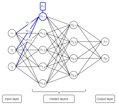
Deep Feed Forward Neural Network (DFF) is the most common type of neural network. Its structure includes an input layer, output layer, and at least one hidden layer containing neurons, weights, bias, and an activation function. Data flows from the input to the output (a forward pass) via a series of calculations (described later in detail). The image below represents the structure of a DFF neural network:

Convolutional Neural Network

Convolutional Neural Networks (ConvNet or CNN) is an extended form of DFF and is primarily used for feature extraction from a grid-like matrix dataset. ConvNets are very powerful tools, typically used for image recognition or signal processing. In SysCAD, we have used ConvNet for dynamic time-based process simulation with great success, with much better performance (lowest loss) than DFF using the same training and validation dataset.

ConvNet has many layers which include an input layer (typically a 2D or greater dimension matrix-type), one or more convolutional and pooling layers, followed by a fully-connected layer represented by a DFF. Essentially a ConvNet is a DFF with additional pre-processing steps to simplify and summarise the input data.

How do Neural Networks Work?

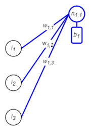
A neural network is a network of connected neurons. Each connection is given a weight, and each neuron in the network calculates the sum of weighted inputs, plus a bias. The calculated value is then subject to an activation function. The output value from each neuron is then sent to neurons in the next layer, and so on. The mathematical computation done for each node is represented by the formula:

[math]\displaystyle{ output= f_{act}\left({\sum_{i=1}^{n_{inputs}}({input_i*weight_i}}) +bias\right) }[/math]

Neural Network Parameters

Neural Network parameters are the learnable / trainable values within the network. The final values of these parameters are obtained by an optimisation process (training or fit) where successive adjustments to these values are made in order to minimise the error (or loss) between the predicted values of the output layer and the true values for each sample in the dataset.

For a DFF network, these are the weights and biases which impact the behaviour of each neuron. Weights are usually randomised and biases are zeroed before the learning session begins. Together with an activation function, they allow the model to propagate forward and produce an acceptable output.

Weight: The weight is multiplied by the input value entering the node. The weights represents the strength of a node connection.

Bias: The output value from a neuron can be shifted using a bias. The bias can be compared to the y-intercept in a linear equation.

For a ConvNet, there are additional trainable parameters. These are the coefficients of a kernel which are used to extract features from the input matrix and also reduce the dimensions or size of the inputs.

Kernel: This is a matrix or set of matrices with a smaller size than the input layer, used to calculate the dot product between a section of the input layer and the kernel. The kernel is displaced, sweeping through the input matrix and calculating the dot product again, repeating until the entire input is processed. This produces a new layer called an activation map or feature map which contains only the dot products and is typically of a smaller dimension than the input matrix. Kernels act as filters, identifying features, and simplifying and summarising the input data into to more computationally manageable chunks. The values of this kernel matrix need to be optimised during the training process.

Neural Network Hyperparameters

Below are some of the hyperparameters that can be modified when setting up a neural network model. These are not trainable parameters but rather design parameters defining the structure or makeup of the NN model. Initially, one might not know how many layers, or neurons per layer, are going to result in the lowest validation loss. Similarly, the use of one or more convolutional layers, number of kernels (each convolutional layer might have several kernels), the size of the kernel window, whether to use or not pooling layer at all, etc.

The process by which one determines the final NN design is often referred to as hyperparameter tuning or optimisation and involves running parametrically, several combinations of designs, training each NN model using the same dataset and evaluating which combination of hyperparameters results in the lowers training and validation losses.

Neuron Count: A neuron in a neural network is where the sum of the weight multiplied by the input is computed and a bias is added. A large number of neurons can be used, however some popular number of neurons used are 32, 64 or 128 (aligning with computer hardware for efficient calculation).

Activation Function: The net output from the neuron is passed through an activation function. The type of activation function can be selected as hyperparameter by the user, whereas the weights and biases are adjusted during the training process. The choice of activation function(s) depends on the problem you are trying to solve. Some examples are Rectified linear function (ReLU), SoftMax and Sigmoid Function. The purpose of this activation function is to introduce non-linearity into the output of a neuron, making the model much more versatile and capable of modelling very complex problems despite the simple mathematical structure.

Input Layer: The input layer is the first layer where all the inputs are given for the model. The number of neurons for the input layer depends on the number of features or inputs in the dataset.

Hidden Layer(s): The hidden layer obtains the data from the input or previous layers. In the model there can be as many hidden layers as necessary and each hidden layer can have a different number of neurons.

Output Layer: The output layer is the the last layer of the neural network. The number of neurons in the output corresponds to the number of outputs or variables representing true values there are.

Loss: Loss is the metric used during the optimisation or training process. Depending on the type of model, different loss functions can be defined such as Categorical Cross-Entropy and Binary Cross-Entropy (for categorical-type problems) and Mean Squared Error or Mean Absolute Error (for regression-type problems).

Optimiser: These are crucial in assisting the network in learning to generate ever-better predictions during training. Optimiser routines assist in determining the optimal set of model parameters (weights and biases) so that the model can generate the best results for the problem it is solving. There are many types of optimisers that can be used such as stochastic gradient descent (SGD), SGD with decay, SGD with momentum, AdaGrad (Adaptive Gradient), RMSProp (Root Mean Square Propagation), and AdaM (Adaptive Momentum). AdaM is the most widely used optimiser as is often capable of finding the global minimum and avoiding getting stuck in local minima.

Learning Rate: The learning rate determines the amount that the model will change in response to the estimated error every time the model weights are changed. This is similar to the gain in a PID Controller. Choosing the correct value for learning rate is important because if the learning rate is too small then this can result in the training process being too long or it could get stuck. However, if the value is too large then it could result in a sub-optimal set of weights. Learning rate values range between 0 and 1.

Epochs: In neural networks a forward and a backward pass together is counted as one iteration during the training sessions. The number of epochs may be interpreted as the total number of iterations the algorithm has made across the training dataset.

The additional parameters below are only for Convolutional Neural Networks:

Convolutional Layer: In the convolutional layer the dot product between two matrices corresponding to a section of the input layer and the kernel is preformed. The kernel slides across the height and width of the dataset, each time performing a dot product, producing an activation map. Typically an activation function, similar to that used for DFF NN, is then applied to the activation map.

Pooling Layer: The pooling layer summarises statistics of nearby outputs from the activation map. There are different types of pooling functions that can be used such as average rectangular neighbourhood, L2 norm of the rectangular neighbourhood, or max pooling. Max pooling is the most popular type of pooling function.

Creating a Neural Network

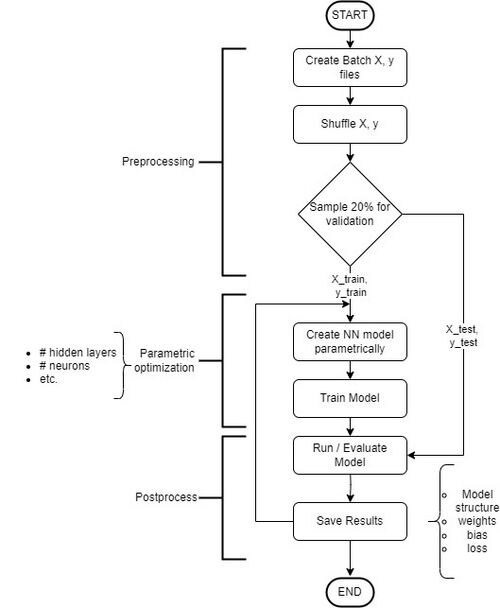
The following is a high-level overview of the steps required to set up and train a neural network, summarised in the flowchart to the right. A detailed walkthrough of this process will be presented in Part 2.

1. Source Data: In order to create and run a neural network you first need to collect data for all the inputs and outputs you require. For example, process data such as temperature, pressure, input flows, tank levels, etc.
2. Preprocessing: It is generally good practice to pre-process the data, such as by shuffling and scaling. To avoid overfitting, it is also recommended to set aside about 20% of the data collected for validation while the remaining 80% is run through the NN during training.
3. Parametric Optimisation: Many different tools can be used to design the NN structure and obtain the final optimised parameters. For example, in Python some available tools include TensorFlow, TensorBoard and PyTorch. Other programming languages that can be used are R, Java, C++, and many more.
4. Postprocessing: Hyperparameters should also be adjusted to find the optimal NN structure (lowest loss). For DFF, these include learning rate, epochs, hidden layers, and neurons. For ConvNet there is also time window size, convolutional layers, convolutional filters, size of kernel, and pooling layer size.
5. Save Results: After parameter tuning and hyperparameter optimisation, it is of course very important to save the NN model structure including the final weights and biases for later use.

Neural Networks in SysCAD

There are several ways SysCAD can be combined with Machine Learning and Neural Networks.

• SysCAD as the Data Source: Using a detailed calibrated SysCAD model of a process, we could generate a large dataset by running scenarios covering a wide range of input conditions and generating the corresponding outputs. This data could then be used to train a NN model.
• NN as a Unit Model within SysCAD: We can incorporate a predefined NN model as a unit operation within a SysCAD project. Here the dataset used for training and validation has been generated externally (or from another SysCAD model as above). SysCAD can use a NN API to load the optimised NN parameters and calculate the output of a NN model at each SysCAD iteration while interacting with other SysCAD unit models, in the form of a controller or reactor unit model. In the simplest case, custom PGM code could be implemented to perform the NN forward pass. Alternatively, as demonstrated in the example below, a custom unit model running a development C++ NN API can be used directly in place.

SysCAD NN API

The SysCAD NN API is currently in development. The API is a set of C++ dynamic libraries (DLL) that enable SysCAD to:

• Load and run an optimised DFF or ConvNet model from file
• Run a Mass Balance Reactor unit model based on optimised NN parameters

The optimised parameters for the DFF or ConvNet models can be generated using the same SysCAD NN API outside of SysCAD, or some of the publicly available libraries. In Part 2 of this series we will show in detail how this process works using TensorFlow.

Once NN model parameters are loaded, the NN API is used by a SysCAD General Controller or reactor unit model, providing the necessary inputs to the NN model, calculating the outputs, and transferring those outputs back to the SysCAD model.

Mass Balance Neural Network Reactor

The Mass Balance Reactor unit model uses a NN to model chemical reactions within a process, converting input reactants to output products. Critically, this must be done while maintaining mass balance.

Defining the Problem

As an example, let's look at the methane combustion system CH₄ + O₂ which produces a range of species (including CO₂, CO and H₂O). A mass balance system can be defined by system components (SC) and phase constituents (phC), in this case the elements and species respectively. The SC and phC are related by a stoichiometric matrix ([math]\displaystyle{ S }[/math]) (i.e. the elemental composition of each species). A set of independent orthonormal basis vectors ([math]\displaystyle{ \vec{b_j} }[/math]) can be obtained for the [math]\displaystyle{ S }[/math] matrix by calculating the nullspace of [math]\displaystyle{ S }[/math]. The number of vectors ([math]\displaystyle{ J }[/math]) represents the degrees of freedom (or nullity) of the system. Any mass transfer in the system (generation or consumption) with no net overall mass change can be calculated by a set of transformation coefficients ([math]\displaystyle{ \lambda_{j} }[/math]):

[math]\displaystyle{ \vec{y_{out}}[moles]= \vec{y_{in}} + \sum_{j=1}^{J} \lambda^{}_{j} \cdot \vec{b_j} }[/math]

The stoichiometric matrix and the set of basis vectors for the system are shown below. Here, only the gas phase is considered, consisting of 6 phase constituents (species, the rows in [math]\displaystyle{ S }[/math]) and 3 system components (elements, the columns in [math]\displaystyle{ S }[/math]).

It is important to note that there are infinite sets of possible independent basis vectors. For this example, a RREF (reduced row echelon form) of the basis vectors was chosen for convenience as it makes it easy to calculate the transformation coefficients given a training data set.

[math]\displaystyle{ \ \ \ O \ \ \ C \ \ \ H }[/math]

[math]\displaystyle{ S =\matrix{H_2 \\ CH_4\\ O_2\\ H_2O\\ CO\\ CO_2\\} \pmatrix{ 0 & 0 & 2 \\ 0 & 1 & 4 \\ 2 & 0 & 0 \\ 1 & 0 & 2 \\ 1 & 1 & 0 \\ 2 & 1 & 0 \\} \quad \quad \vec{b} = \pmatrix{1 & 0 & 0 \\ 0 & 1 & 0 \\ 0 & 0 & 1 \\ -1 & -2 & 0 \\ -1 & -4 & 2 \\ 1 & 3 & -2} }[/math]

Note that each of the basis vectors ([math]\displaystyle{ \vec{b_j} }[/math], i.e. the columns in [math]\displaystyle{ \vec{b} }[/math]) represent values for a stoichiometrically balanced reaction. E.g. for the first column: 1 H₂ + 1 CO₂ ⇔ H₂O + CO. The three vectors represent the degrees of freedom for the system, i.e. any overall reaction the system can be represented by some combination of these three reactions.

The overall mass balance equation for this CH₄ + O₂ combustion system is then:

[math]\displaystyle{ \pmatrix{{y}_{H_2} \\{y}_{CH_4} \\{y}_{O_2} \\{y}_{H_2O} \\{y}_{CO} \\{y}_{CO_2}}_{out} = \pmatrix{{y}_{H_2} \\{y}_{CH_4} \\{y}_{O_2} \\ {y}_{H_2O} \\{y}_{CO} \\{y}_{CO_2}}_{in} + \lambda_{1} \pmatrix{1 \\ 0 \\ 0 \\-1 \\-1 \\1} + \lambda_{2} \pmatrix{0 \\1 \\0 \\-2 \\-4 \\3} + \lambda_{3} \pmatrix{ 0 \\0 \\1 \\0 \\2 \\-2} }[/math]

For any feed stream vector of species [math]\displaystyle{ \vec{y_{in}} }[/math], an arbitrary set of transformation coefficients [math]\displaystyle{ \lambda_i }[/math] will produce a product vector [math]\displaystyle{ \vec{y_{out}} }[/math] with mass and element balance strictly conserved. However, while the total mass of the system is conserved, it does not guarantee that all phase constituents will have positive mass. That problem needs to be addressed by improving accuracy of the model and by implementing mechanisms to ensure all output masses are positive (constrained mass balance).

The problem now is to find a set of [math]\displaystyle{ \lambda_j }[/math] values given a known set of input species, T and pressure. This is similar to solving a thermodynamic equilibrium problem for the system, where the thermodynamic model (e.g. GFEM or TCE) can calculate the output species representing the most stable state. However, in this case, we will use a trained Neural Network to find [math]\displaystyle{ \lambda_j }[/math] values for each input set. Here, the training and validation datasets are generated using an equilibrium thermodynamics model (but could equally be done from experimental results or operational measurements).

When creating the NN, true values for [math]\displaystyle{ \lambda }[/math] need to be calculated for each set of input species, T, P and true output composition. This can be done using the following equation for [math]\displaystyle{ \lambda_{1} }[/math], [math]\displaystyle{ \lambda_{2} }[/math] and [math]\displaystyle{ \lambda_{3} }[/math] (thanks to the simplified form of the RREF basis vector):

[math]\displaystyle{ \lambda_{1}= y_{1,out}-y_{1,in}=y_{H_2,out}-y_{H_2,in} }[/math]

[math]\displaystyle{ \lambda_{2}= y_{2,out}-y_{2,in}=y_{CH_4,out}-y_{CH_4,in} }[/math]

[math]\displaystyle{ \lambda_{3}= y_{3,out}-y_{3,in}=y_{O_2,out}-y_{O_2,in} }[/math]

Training the Model

Once the input and true output dataset is collected or generated, this can be used to train a NN model. For this example, a set of 2000 random combinations of input amounts for all 6 phase constituents and random temperature between 300 and 6000 K was generated as input/training data.

NNs typically expect input values between 0 and 1. As such, the input amounts were normalised so that the sum of all inputs added to 1, while the temperature was divided by the maximum temperature used in this example (6000 K). This ensures that the NN model will work for any set of inputs and temperature, as long as normalised and scaled inputs are provided before performing a forward pass through the trained model. This step is integrated into the NN API.

To train the neural network, almost any programming language can be used. Various parameters such as epochs, hidden layers, type of optimiser, learning and decay rates were adjusted to determine the optimal set of weights and bias, and the structure of the neural network.

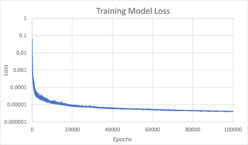
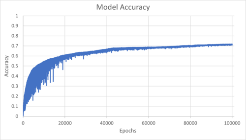
For this example, the best hyperparameters were 2 hidden layers, 64 nodes for the hidden layers, Adaptive Momentum (AdaM) for the optimiser, a learning rate of 0.006, a decay rate of 0.005, and 100000 epochs. The training results for [math]\displaystyle{ \lambda_{1} }[/math], [math]\displaystyle{ \lambda_{2} }[/math] and [math]\displaystyle{ \lambda_{3} }[/math] are shown in the animation below. The outputs from the initially randomised weights are shown at iteration 0, improving through to 100000 epochs. As can be seen, results from the last iteration were very accurate!

The Loss and Accuracy throughout the training was also calculated. As shown in the following graphs, the overall loss was ~1e-5 and the accuracy was ~70% after 100000 epochs.

Depending on the type of Neural Network (categorical, binary or regression), there are different methods to calculate loss and accuracy. Note that the NN training process considers only the loss. Accuracy is usually an arbitrary measure for ease of interpretation by the user.

To calculate the Loss, we determined the Mean Squared Error (MSE) between the true ([math]\displaystyle{ y }[/math]) and predicted ([math]\displaystyle{ \hat{y} }[/math]) values for each of the [math]\displaystyle{ K }[/math] samples (2000 in this case) for each of the [math]\displaystyle{ J }[/math] outputs (3 transformation coefficients [math]\displaystyle{ \lambda }[/math]):

[math]\displaystyle{ L = \frac{1}{K\cdot J} \sum_{k=1}^{K} \sum_{j=1}^{J} \left(y_{k,j} - \hat{y}_{k,j}\right)^2 }[/math]

To calculate the Accuracy for the regression model, we assess each individual sample [math]\displaystyle{ k }[/math] for each output [math]\displaystyle{ j }[/math], and assign a binary value (true/false) if the model is accurate or not. In this case, we compared the absolute difference between the true ([math]\displaystyle{ y }[/math]) and predicted ([math]\displaystyle{ \hat{y} }[/math]) values with a specified threshold [math]\displaystyle{ \varepsilon }[/math]:

[math]\displaystyle{ a_{k,j} = \begin{cases} 0 & \text{if } |y_{k,j} - \hat{y}_{k,j}| \geq \varepsilon_j \\ 1 & \text{if } |y_{k,j} - \hat{y}_{k,j}| \lt \varepsilon_j \end{cases} }[/math]

The choice and definition of threshold depends on the application and the problem that is being solved. This may be some defined level of permissible/acceptable error. In this case, in order to keep the outputs comparable, a threshold [math]\displaystyle{ \varepsilon_j }[/math] is defined for each output [math]\displaystyle{ j }[/math], as an arbitrary fraction of the standard deviation [math]\displaystyle{ \sigma }[/math] of each set of true values [math]\displaystyle{ y_j }[/math]:

[math]\displaystyle{ \varepsilon_j = \frac{\sigma_{y_j}}{100} }[/math]

The total accuracy (i.e. the fraction of "accurate" results per our definition) is then simply the average of all individual accuracy values across all samples and outputs ([math]\displaystyle{ \overline{a}_{k,j} }[/math]).

Using the Model

Once the model has been trained, the NN API is used to load the optimised parameters for use by the SysCAD Mass Balance Reactor.

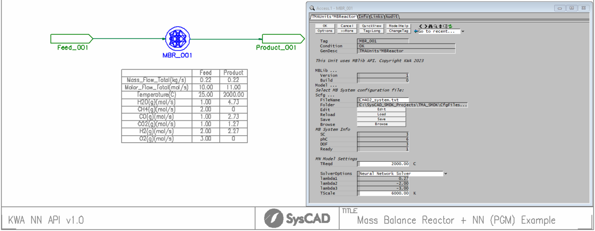
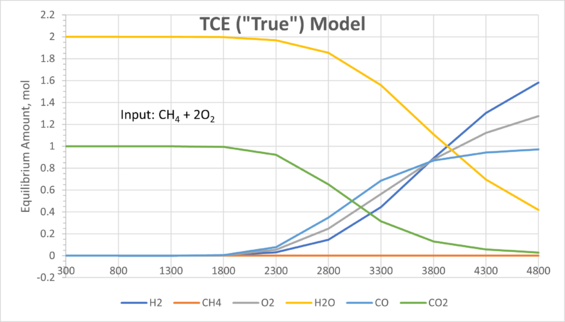
A validation dataset was used to test the model. For ease of visualisation, fixed inputs (1 mol of CH₄ and 2 mol of O₂) were tested across a range of temperatures:

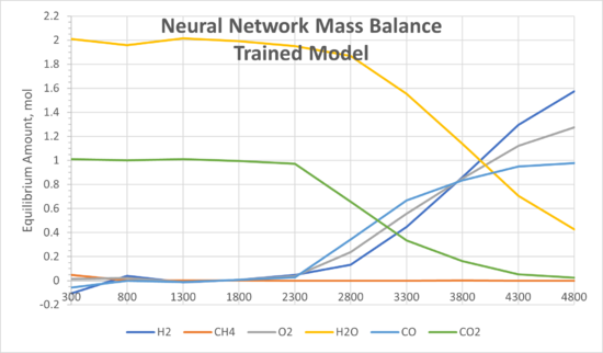
On the left are results from a SysCAD TCE model (considered as the true values). On the right are results from the Mass Balance Reactor Model using the optimised NN. Comparing both models, the results are in very good agreement. As demonstrated, NNs can be used in various different scenarios for process simulation given a good set of supervised data is available.

Advantages and Disadvantages

So, after looking at this high-level description of supervised machine learning and our mass balance example for the combustion of methane, you might be asking, is it all worthwhile? Is it more advantageous than just using a GFEM or TCE model or another high definition model? In some cases, yes it is!

There are various pros and cons to using Neural Networks in process modelling:

Advantages:

• Depending on the amount and quality of training data, NNs can achieve highly accurate results.
• Due to their simple mathematical structure, NNs are fast to compute since they don't require an iterative process or detailed calculations once trained. Compared to a highly complex and non-ideal thermodynamic solver, a NN model can be seen as an accelerator. The slower (but highly accurate) thermodynamic solver is used to pre-train the NN, and then when embedded in a large model with multiple recirculation streams, the gain in speed can drastically reduce the overall computation time.
• NNs can be used for a wide range of applications. They are used to model non-linear relationships, for pattern recognition, and classification problems. This versatility allows us to add more features to a model that would otherwise be difficult to incorporate.
• NN models can be used for forecasting model outputs. For example, in a time-dependent dynamic model, one trained NN model could be used to predict the immediate process outcome, while another acts in parallel (using separate trained data) to predict the outcome at some future time. This model would probably have lower accuracy but the correct trend, and would act as an early warning indicator to support decision-making.

Disadvantages:

• Requires a large, cleaned and labelled dataset for supervised learning. Depending on the problem you solving, this may take a very long time to collect.
• Training can be difficult and lengthy. Similar to controller tuning, it is often more of an art than a science.
• NNs often have limited extrapolation capability and may not perform well outside of the training dataset range. This should be addressed in training, ensuring a proper balance between training and validation datasets. It is easy to fall into the trap of overtraining a model, making it too rigid and compromising the performance of the model outside of the training dataset.
• Despite the flexibility that ML and NN models provide, there are also certain constraints. For example, if we decided to add more phase constituents or system components to our methane combustion model, we would need to generate a new training and validation dataset and refit the model before it could be used in SysCAD.

What's Next?

In the next part of this series, we will walk through the details of creating a NN model for steady-state process simulation from scratch, including:

• Creating a GFEM model to generate the training and validation dataset
• Training the model and optimising the hyperparameters
• Implementing the newly-trained model in a SysCAD project

References

• R. Bagheri (2020) "An Introduction to Deep Feedforward Neural Networks", Towards Data Science, Medium
• J. Brownlee (2020) "Understand the Impact of Learning Rate on Neural Network Performance", Machine Learning Mastery
• I. Goodfellow, Y. Bengio and A. Courville (2018) "Chapter 9: Convolutional Networks" in Deep Learning, MIT Press, pp. 326–366
• K. Nyuytiymbiy (2020) "Parameters and Hyperparameters in Machine Learning and Deep Learning", Towards Data Science, Medium
• M. Mishra (2020) "Convolutional Neural Networks, Explained", Towards Data Science, Medium

---

First Posted: 14 February 2024

Reference Build: 139.34613

For questions or feedback, please contact us at [email protected].