Bayer3 Species Model Theory

Navigation: Models ➔ Alumina Models ➔ Bayer3 Species Model ➔ Bayer3 Species Model Theory

Bayer3 Species Model	Species Model Theory	General Discussion

Latest SysCAD Version: 19 March 2024 - SysCAD 9.3 Build 139.35102

Related Links: Precipitation3, Species Models

---

Nomenclature and Units

The calculations for liquor and slurry densities, heat capacity and boiling point elevation are evaluated using the following formulae:

The variables used in the calculations are described below:

A	=	Sodium Aluminate NaAl[OH]4 concentration, expressed as grams of Al2O3/L liquor @ slurry temperature
C	=	Caustic Soda concentration in NaOH + NaAl[OH]4, expressed as grams Na2CO3/L liquor @ the slurry temperature
A25	=	Sodium Aluminate NaAl[OH]4 concentration, expressed as grams of Al2O3/L liquor @ at 25°C.
C25	=	Caustic Soda concentration in NaOH + NaAl[OH]4, expressed as grams Na2CO3/L liquor @ 25°C.
T	=	Temperature in °C
Tk	=	Temperature in K
TOC25	=	Total Organic carbon (Na2C5O7 + Na2C2O4) expressed as g/L Carbon @ 25°C;
TNa	=	The sum of all sodium salts, caustic, sodium aluminate, carbonate, organics, NaCl, Na2SO4, sodium silicate all expressed as Na2CO3 @ 25°C. The engineering units for this is Concentration (mass/mass) wt%. [math]\displaystyle{ \mathbf{\mathit{\left([Na_2CO_3] + \begin{pmatrix}\dfrac{[NaOH]}{2\times MW_{NaOH}} + \dfrac{[NaAl[OH]_4]}{2\times MW_{NaAl[OH]_4}} + \dfrac{[Na_2C_2O_4]}{MW_{Na_2C_2O_4}} \\ +\dfrac{[Na_{org}]}{MW_{Na_2C_5O_7}} + \dfrac{[NaCl]}{2\times MW_{NaCl}}+\dfrac{[Na_2SO_4]}{MW_{Na_2SO_4}} \\ +\dfrac{[Na_2SiO_3]}{MW_{Na_2SiO_3}}+\dfrac{[NaF]}{2\times MW_{NaF}} \end{pmatrix} \times MW_{Na_2CO_3}\right)\times \dfrac{100}{L_m}}} }[/math] Lm = Liquor mass flow (engineering units need to be the same as individual salts in the equation.)
TAl2O3	=	Total concentration (mass/mass) wt% of Alumina. [NaAl[OH]4] = NaAl[OH]4 mass flow, Lm = Liquor mass flow [math]\displaystyle{ \mathbf{\mathit{T_{Al203}= [NaAl[0H]_4] \times \left( \cfrac{MW_{Al_2O_3}}{2\times MW_{NaAl[OH]_4}}\right)\times \cfrac{100}{L_m}}} }[/math]

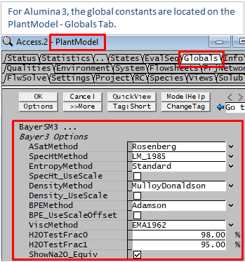
Method Selection for Property Calculations

For many of the property calculations described below, more than one method is available. The user can make a selection of which method should be used. This is applied globally, so you cannot use different methods in different areas in the same project. The method is selected globally from the View - PlantModel access window Globals Tab as illustrated below.

NOTE For very dilute solutions, ie, solutions containing >=98% water (or H2OTestFrac0), SysCAD will automatically use the "Standard Species model" to calculate its properties. This includes Density, Heat Capacity Saturation T and P etc. For solutions >=95%(or H2OTestFrac1) water and <=98% (or H2OTestFrac0) Water, a proportional result of "Bayer3 and Standard" Species properties are used to calculate the stream properties. Boiling Point Elevation must be greater or equal to 0.

See Global Properties Calculation Method Selection for more information.

Density Calculations

Mulloy-Donaldson equation. - This is based on a correlation for density at standard conditions (25°C) and a correction for temperature.

NOTE: for very dilute solutions, i.e. >98% water, this density equation is not used. SysCAD will use the Standard Species model to calculate its properties.

Liquid SG

Function	Equation	Notes
Liquid SG at Temperature	[math]\displaystyle{ LSG_T =LSG_{25} \big\{ 1 - \left[e_0 \times 0.85(T - 25) \right] - \left[e_1 \times 0.85(T - 25)^2 \right] \big\} }[/math]	where: LSG25 is the liquid SG @ 25°C e0 = 0.0005021858 e1 = 0.0000011881
Liquid SG at 25°C	[math]\displaystyle{ LSG_{25} = \begin{pmatrix} a_0 \, + \left(b_0 \, T_{Na} \, + \, b_1 \, T_{Na}^2 \, + \, b_2 T_{Na}^3 \, \right) \\ + \left(c_0 \, T_{Al_2O_3} \, + \, c_1 \, T_{Al_2O_3}^2 \,+ \,c_2 \, T_{Al_2O_3}^3 \, \right) \, \\ + \, \left(d_0 \, T_{Na} \times T_{Al_2O_3} \, \right) \end{pmatrix} }[/math]	Where: TNa = Total concentration (mass/mass) wt% of Sodium, reported as Na2CO3. (See Nomenclature and Units) TAl2O3 = Total concentration (mass/mass) wt% of Alumina. (See Nomenclature and Units) a0 = 0.982 c0 = 0.00208035 b0 = 0.01349855 c1 = 0.00004113 b1 = -0.00024948 c2 = -0.00000728 b2 = 0.00000273 d0 = 0.00033367

Slurry SG

Slurry SG at Temperature	[math]\displaystyle{ \mathbf{\mathit{SL_{{SG}_{T}}=\cfrac{SolidsMass+LiquidsMass}{SlurryFlow}}} }[/math]
Slurry Flow at Temperature	[math]\displaystyle{ \mathbf{\mathit{SlurryFlow=\cfrac{SolidsMass}{SolidsSG}+\cfrac{LiquidsMass}{LSG_T}}} }[/math]
Slurry SG at 25°C	[math]\displaystyle{ \mathbf{\mathit{SL_{{SG}_{25}}=\cfrac{SolidsMass+LiquidsMass}{SlurryFlow\ 25^{\circ} C}}} }[/math]
Slurry Flow at 25°C	[math]\displaystyle{ \mathbf{\mathit{SlurryFlow=\cfrac{SolidsMass}{SolidsSG}+\cfrac{LiquidsMass}{LSG_{25}}}} }[/math]

Heat Capacity Calculations

NOTE: for very dilute solutions, i.e. >=98% (H2OTestFrac0) water, these Cp equations are not used. SysCAD will use the Standard Species model to calculate its properties.

See Selecting alternative methods for Property Calculations

Liquid Heat Capacity

Methods	Equation	Notes
LM_1985	[math]\displaystyle{ Cp_L=4.184 \left(K_1 + K_2 T + K_3 T^2\right) }[/math] where [math]\displaystyle{ K_1 = 0.99639 - 3.90998e^{-4}C_{25} - 5.3832e^{-4}A_{25} + 2.46493e^{-7}C_{25}^{2} + 5.7186e^{-7}C_{25} \times A_{25} }[/math] [math]\displaystyle{ K_2 = -1.51278e^{-4} - 1.86581e^{-7} A_{25} - 1.07766e^{-7} C_{25} }[/math] [math]\displaystyle{ K_3 = 2.1464e^{-6 } }[/math]	(Langa method from Light Metals 1985)
Mulloy Donaldson	[math]\displaystyle{ \mathbf{\mathit{Cp_L=\begin{pmatrix}1.0275057375729-0.020113606661083 T_{Na_2O}\\ +0.001081165172606 T^2_{Na_2O}-0.000022606160779 T^3_{Na_2O}\\ -0.004597725999883 T_{Al_2O_3}-0.000001053264708 T^2_{Al_2O_3}\\ -0.00000218836287 T^3_{Al_2O_3}\end{pmatrix}\times 4.184}} }[/math] where [math]\displaystyle{ \mathbf{\mathit{T_{Na_2O}=T_{Na} \cfrac{MW(Na_2O)}{MW(Na_2CO_3)}}} }[/math]	This is scaled for dilute liquors where TNa2O as liquid weight % is less than 0.19.

Solids and Vapours Heat Capacity

Solids Cp (Cp_s) and Vapours Cp (Cp_v) are calculated from Cp values as given in the species database, using Standard Species Model.

Stream Heat Capacity

• [math]\displaystyle{ \mathbf{\mathit{Cp=\cfrac{SolidsMass*Cp_s+LiquidsMass*Cp_L+VapoursMass*Cp_V}{SolidsMass+LiquidsMass+VapoursMass}}} }[/math]

Entropy

Methods	Equation	Notes
Standard	Entropy values are not calculated by the Bayer model.	Calculated by the Standard Species Model.
LM_1985	[math]\displaystyle{ S(T) = S^{25} + \int_{298.15}^T \cfrac{Cp}{T} dT }[/math]	Based on the LM_1985 specific heat equation Please see Entropy for some caution notes on using this method.

Boiling Point Elevation

See Selecting alternative methods for Property Calculations

Methods	Equation	Notes
Dewey Equation2	[math]\displaystyle{ \mathbf{\mathit{BPE=\left(\begin{matrix}&0.00182+0.55379\times \left(\frac{M}{10}\right)^7+0.0040625\times M\times T_K\\ &+\frac{1}{T_K}\times \left(-286.66\times M+29.919\times M^2+0.6228\times M^3\right)\\ &-0.032647\times M\times \left(M\times \frac{T_K}{1000}\right)^2+\left(\frac{T_K}{1000}\right)^5\\ &\times \left[5.9705\times M-\left(0.57532\times M^2\right)+\left(0.10417\times M^3\right)\right] \end{matrix}\right)}} }[/math]	M is the Total Molality of the solution, calculated using the following species: NaAl[OH]4, NaOH, Na2CO3, NaCl, Na2SO4, Na2C5O7 (or equivalent), Na2C2O4, Na2SiO3 and NaF. Tk is the liquor temperature in K. In the original Dewey paper, Tk is the saturated temperature for the liquor , see the notes on Boiling Point Elevation Discussion. The Dewey relation correlates the liquor boiling temperature with the water boiling point at liquor saturation pressure. Dewey All Liq is a variation of this, where instead: [math]\displaystyle{ M }[/math] is the SysCAD calculation of total Molality using ALL liquid species.
Adamson Equation	[math]\displaystyle{ \mathbf{\mathit{BPE=\left(\begin{matrix}&0.007642857+0.006184282X+2.92857e^{-5}*T\\ &+0.00010957X^2-3.80952e^{-8}T^2+0.000208801.XT\\ &-8.61985e^{-10}X^3-8.61985e^{-10}T^3\\ &+1.7316e^{-10}XT^2-2.49763e^{-7}X^2T\end{matrix}\right)}} }[/math]	X = Total Soda concentration expressed as g/L Na2O @ 25°C T = Temperature in °C. T is the saturated temperature for the liquor, see the notes on Boiling Point Elevation Discussion. The Adamson implementation correlates the liquor boiling temperature with the water boiling point at liquor saturation pressure. Constants in the above equation were determined by data fitting of published Adamson data.

Optional Scale and Offset

A scale and/or offset can be globally applied to the BPE value calculated by the selected BPE method. This is specified in Plant Model on the Globals Tab page - Global Properties Calculation Method Selection.

Saturated Alumina Concentration

Function	Equation	Notes
Rosenberg-Healy3	[math]\displaystyle{ \mathbf{\mathit{A^{*} = \cfrac{0.96197 C_{25}} {1+\cfrac{ 10 ^{\left(\cfrac{\alpha_o \sqrt{I}} {1+ \sqrt{I}} \right)- \alpha_3 \; I \; - \; \alpha_4 \; I^{\tfrac{3}{2}} \; }} {{exp \left({\cfrac{\Delta G_{rxn}}{RT}}\right)}}}}} }[/math]	Where [math]\displaystyle{ \alpha_0 }[/math] [math]\displaystyle{ \alpha_3 }[/math] [math]\displaystyle{ \alpha_4 }[/math] -9.2082 -0.8743 0.2149 [math]\displaystyle{ \Delta G_{rxn} }[/math] is the Gibbs energy of dissolution (-30960 kJ/kmol) R is the Universal Gas Constant
Ionic Strength	[math]\displaystyle{ \mathbf{\mathit{I=\left(\begin{matrix}&0.01887C_{25}+\cfrac{k_1\left[NaCl\right]}{MW(NaCl)}+\cfrac{k_2\left[Na_2CO_3\right]}{MW(Na_2CO_3)}\\ &+\cfrac{k_3\left[Na_2SO_4\right]}{MW(Na_2SO_4)}+k_4 \times 0.01887TOC_{25}\end{matrix}\right)}} }[/math]	Where k1 k2 k3 k4 0.9346 2.0526 2.1714 1.6734 Concentration of salts and carbonate are @ 25°C.

User Specified Parameters

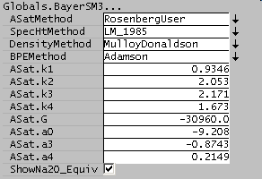
The constants in the Rosenberg-Healy equation may be specified by the user by selecting the RosenbergUser option: [math]\displaystyle{ \alpha_0 }[/math] = ASat.a0 etc.

Oxalate Equilibrium

See Selecting alternative methods for Property Calculations

Calculates the solubility equilibrium concentration (g/L) of sodium oxalate, based on stream properties. Result is limited between 0 g/L and the solubility in water (see below).

Methods	Equation	Notes
Method 1: Burnt Island	[math]\displaystyle{ \mathbf{\mathit{OxEquil=7.62 \times \operatorname{Exp}\left[ \begin{matrix} 0.012T-\left(\cfrac{MW_{Na_2O}}{MW_{Na_2CO_3}}\right) \\ \times \left(0.016C_{25}+0.011\cfrac{Qm_{Na_2CO_3}} {Qv}\right) \end{matrix} \right]}} }[/math]	Qv = Volume flowrate (m3/s) of liquor at 25 °C QmNa2CO3 = Mass flowrate (kg/s) of sodium carbonate T = temperature in °C Note: This is the original equation used in SysCAD, developed by British Aluminium Burnt Island refinery. There is no further references for the equation and it should be used with caution.
Method 2: Beckham Grocott4	[math]\displaystyle{ \mathbf{\mathit{OxEquil=MW_{Na_2C_2O_4} \times \operatorname{Exp}\left[\begin{matrix} \cfrac{-1166.4}{T_K} + 0.511\operatorname{ln}T_K \\ + 7e^{-5}T_C{^2} - 8e^{-6}(C_{25}-100)^2 \\ + 0.0173 \left(\cfrac{C_{25}}{A_{25}} \right)^2\\ -1.7252\operatorname{ln}\left( Term1 \right)\end{matrix}\right]}} }[/math] Where: [math]\displaystyle{ Term1 =\begin{pmatrix} 0.0482C_{25} \, + \, 0.0248Carb_{25} \, - \, 0.0171A_{25} \, + \, 0.054NaCl_{25} \\ + \, 0.0214Na2SO4{_{25}} \, + \, 0.07NaF_{25} \, + \, 0.08TOC_{25} \, \end{pmatrix} }[/math]	TK = Temperature in K TC = Temperature in °C C25 and Carb25 as g/L Na2CO3 A25 as g/L Al2O3 TOC25 as g/L C Notes: The formula was developed using synthetic liquor and tuned to plant liquor. According to the paper, without tuning parameters the equation tends to over-estimate the solubility. At low caustic and aluminate, this model significantly over-estimates solubility. As sodium oxalate is more soluble in pure water than Bayer liquor, the maximum is limited to the calculated solubility in water at the same temperature (see below). This method is available in Build 138 or later.
Solubility in Water5	[math]\displaystyle{ \mathbf{\mathit{OxEquil=0.348763276 \times T_C + 26.09675968}} }[/math]	TC = Temperature in °C Note: This formula is a simple linear regression through available aqueous solubility data5 between 0 - 100°C.

Viscosity

See Selecting alternative methods for Property Calculations

Methods	Equation	Notes
Method 1: EMA1962	[math]\displaystyle{ \mathbf{\mathit{Visc_{Liq}=10^{Power}}} }[/math] [math]\displaystyle{ \mathbf{\mathit{Power=\left(\begin{matrix}0.0857 + T \left(-0.00658 + 2.3e^{-6}T \right)\\ +\cfrac{C_{25}}{1000}*\left[3.56+T \left(-0.0357+1.84e^{-4}T \right) \right]\\ +\cfrac{A_{25}}{1000} \left[ 3.23-C_{25}0.0034\\ -0.1246T+T^{2}(0.00204-1.107e^{-5}T) \right] \end{matrix}\right)}} }[/math]	The correlation (Reference6) is fitted to data with A25 and C25 up to 250 gpl and temperatures up to 80°C. Extrapolating past 80°C fails. Correlation is only valid for liquid phase. Where: The engineering units for viscosity is cP. T is in degrees of Celsius. A@25 is in terms of g/L Al2O3. C@25 is in terms of g/L NaOH.
Method 2: Alexandrov (Alexandrov Viscosity method for Caustic7)	[math]\displaystyle{ \mathbf{\mathit{ Viscosity{solution} = WaterViscosity \times \operatorname{Exp} \left( A \right)}} }[/math] [math]\displaystyle{ \mathbf{\mathit{A = t \times m \left( Term1 + m \left(Term2 + Term3 \times m \right) \right) }} }[/math] [math]\displaystyle{ \mathbf{\mathit{t = \cfrac{T_{0}}{T}}} }[/math] [math]\displaystyle{ \mathbf{\mathit{m = \left(\cfrac{Mass_{NaOH}}{MW_{NaOH}} + \cfrac{Mass_{Aluminate}}{MW_{Aluminate}} \right) \div Mass_{Water} \times 1000}} }[/math] [math]\displaystyle{ \mathbf{\mathit{ Term1 = b_{11} + t \left[ \, b_{21} + t \left( b_{31}+b_{41}\;t \;\right) \, \right] }} }[/math] [math]\displaystyle{ \mathbf{\mathit{ Term2 = b_{12} + t \left(b_{22}+b_{32}\;t \; \right) }} }[/math] [math]\displaystyle{ \mathbf{\mathit{ Term3 = b_{13} + b_{23} \; t }} }[/math]	Reference7 states: Viscosity of solutions at molality up to 3 mol/kg in temperature range from 273 to 548 K and under pressures up to 6 MPa. Please see reference for more information on accuracy of the viscosity prediction. Where: WaterViscosity is calculated at the same pressure and temperature as the solution t is temperature ratio, T is solution temperature in Kelvin, T0 is 293.15 K m is the molality of solution in mol/kg Terms and Constants for the equation are: b11 = 5.7050102e-1 b12 = -2.9922166e-1 b13 = 4.9815412e-2 b21 = 4.9395013e-1 b22 = 3.7957782e-1 b23 = -4.8332728e-2 b31 = -2.0417183 b32 = -7.423751e-2 b41 = 1.1654862
Correction for solids	For Newtonian behaviour (large, rounded particles), Heiskanen and Laapas present [math]\displaystyle{ Viscosity Ratio = \cfrac {\mu_{slurry}}{\mu_{liquid}} = 1 + 2.5 v_s + 14.1 v_s^2 + 0.00273 e^{16v_s} }[/math] where vs is the volumetric fraction of solids in the slurry. This is implemented in the Alumina3 model.	When solids are present the viscosity will be greater than for liquor alone. The behavior may or may not be Newtonian and this will depend on the type of liquor and solids as well as the solids concentration. Particle size and shape will also influence the viscosity. Suspensions of rounded particles over 50 microns will tend to have Newtonian behavior, while irregularly shaped particles exhibit Bingham plastic behavior even at larger particle sizes. There is thus no single correlation that we can use to correct for solids in a liquor; the viscosity will depend on many factors.

CAVEAT: Calculations using the viscosity model supplied should be treated as indicative only and use of the numbers in detailed design should be discouraged. Laboratory testing of liquors should be undertaken to provide accurate viscosity measurements for design of settlers, classifiers and heat transfer equipment.

Viewing Viscosity values

The calculated viscosity can be viewed in SysCAD (streams/contents) by enabling the Transport Properties group, either by

• selecting the "Transport" tickbox from "Plant Model - Views tab page" or
• by pressing the "Include Properties" button on the pipe Qo tab and select "Transport"

  

References

1. Molloy-Donaldson Model
2. Dewey, J.K.L. Boiling Point Rise of Bayer Liquors. Light Metals 1981. The Metallurgical Society of AIME pp 185 -- 197.
3. Rosenberg S.P and Healy S.J. A Thermodynamic Model for Gibbsite Solubility in Bayer Liquors. Fourth International Alumina Quality Workshop. June 1996.
4. Beckham K.R. and Grocott S.C. A Thermodynamically Based Model for Oxalate Solubility in Bayer Liquor. Light Metals 1993 pp 167 -- 172.
5. Söhnel O. and Novotny P. Densities of Aqueous Solutions of Inorganic Substances, Elsevier, Amsterdam, 1985.
6. Extractive Metallurgy of Alumina, 1962.
7. "Equations for Thermophysical Properties of Aqueous Solutions of Sodium Hydroxide" 14th Intl Conf Props Water Steam, Kyoto 2004.