Alumina3 Precip - Full PSD

Navigation: Models ➔ Alumina Models ➔ Precipitation3 ➔ Model Theory (PSD)

Precipitation3	Model Theory - Growth	Model Theory - PSD	Model Options	Data Sections	Dynamic Mode	Batch Operations (Probal)

Latest SysCAD Version: 19 March 2024 - SysCAD 9.3 Build 139.35102

Related Links: Alumina 3 Bayer Species Model, Size Distribution (PSD)

This page describes the theory and behaviour of the PSD option in the Precipitation3 model. This page has been updated to reflect the latest version of SysCAD. If you are using an earlier version of SysCAD, the display fields may look different.

---

Implementation of Basic PSD Processes

The full PSD model implements growth, agglomeration and nucleation mechanisms. The growth equations are identical to those already implemented in the existing yield SSA model, while the Nucleation and Agglomeration equations are (relatively simple) open literature correlations. The underlying theory was originally developed by Hounslow et al^[1].

Particle Size Definition (PSD)

The precipitation PSD method uses the full Size Distribution (PSD) Quality. The present implementation requires geometrically spaced bins, with a size ratio of [math]\displaystyle{ \sqrt[3]{2} }[/math]. For further information on configuring this in your project, see the section Setting up the PSD Definition below.

Notes:

• When calculating particle counts within bins (size intervals) the geometric mean is used.
• When specifying mass in each bin, the smallest bin should be empty. When it is not empty the model gives a warning message and moves this mass into the next bin up.

Growth

The Growth calculation determines the rate at which new material is deposited on the surface of existing seed. Growth calculations generate a growth rate (of the order of 1[math]\displaystyle{ \mu }[/math]/hr), which is the rate at which the radius of a typical particle will increase. (The diameter increases at twice this rate.)

Please refer to Precipitator3 Model Theory for typical growth rate methods. For the PSD model, the same growth equations have been implemented as the existing alumina precipitator.

For some models (Yield type), growth is not predicted directly, instead, the models predict the rate of change of Alumina concentration or A/C ratio given tank conditions such as temperature and caustic concentration. For these models the growth rate corresponding to the predicted yield is calculated and used in the particle balance calculations. Particle Growth increases the total mass of THA in the tank, without changing particle numbers.

The growth calculations are completely compatible with the existing SSA based growth models, so that if the PSD has a specific surface area equal to that in a model run with SSA alone, the yield calculations will be comparable. (There will be minor differences, since PSD mechanisms change the effective surface area, and this might not quite match what is done with the SSA calculation.)

Nucleation

The empirical Misra Nucleation Rate Equation^[2] implemented is:

[math]\displaystyle{ N = k \left(\cfrac{A-A^*}C\right)^2\sigma }[/math]

where

N is the number of particles nucleated per kg slurry per hour

k is a constant dependent on various process conditions, e.g. [math]\displaystyle{ k_{const} \times e^{-E/RT} }[/math] (Input as Misra.Nucleation.Rate with default value ~[math]\displaystyle{ 5 \times 10^8 }[/math] #/m²/h)

A, A* are alumina and saturation concentrations

C is the Caustic concentration

[math]\displaystyle{ \sigma }[/math] is the specific surface area (m²/kg)

NOTES:

• Nucleation is associated with existing particle area - so that if no particles (THA solids) are present, then no nucleation takes place.
• Nucleation increases particle numbers in the smallest sizes. For the present model nucleation places particles in the second smallest bin. Any particles in the smallest bin are ignored - this is intended more as a 'catchall' for particles below the minimum size, and quantifying the distribution of particles in this bin is difficult.

Bound Soda with Nucleation

The precipitation yield includes Growth Yield and Nucleation Yield. By default, the bound soda is calculated based on the total yield. If user wishes to exclude the Nucleation yield from the soda calculation, please uncheck the SodaWithNucleation option on the PSD Tab.

Agglomeration

Agglomeration is the tendency of particles to coalesce to form larger particles. Thus there is no total mass change associated with agglomeration, but a reduction in total numbers of particles and shift of the distribution curve - increasing the mean of the curve and changing the skewness and kurtosis (peakiness).

There are a wide range of agglomeration kernels in use in particle size modelling - both in the open literature and proprietary. The original implementation of the model used the Ilievski size independent kernel (Light Metals, 1982). This assumes that all interactions are equally likely to cause an agglomeration event, and the rate is governed by a single equation depending on temperature and liquor properties. (In Build 139, this original implementation is achieved with selection of Agglom.Kernel.Type Size Independent and Agglom.Rate.Type Supersaturation.)

The user can optionally specify a maximum size above which agglomeration does not occur, via Agglom.Cutoff.

From Build 139, the agglomeration parameters for kernel, rate, collision, etc. have been modularised to allow different combinations of terms and customisation of individual terms. A simplified generalised equation is presented as:

i.e. The change in particle count (per mass of slurry) N at size i, for all sizes j<i, is equal to the product of the interacting particle counts, the agglom kernel, and the total agglom rate (agglom rate plus other corrections, including for collision frequency, slurry density and solids concentration). The total agglom rate represents the chance of a particle interaction resulting in an agglomerate.

• The agglom kernel [math]\displaystyle{ \beta }[/math] is a 2-dimensional array of values (typically presented as a triangular matrix or 3D surface) representing the probability of interaction at each particle size combination, normally a function of particle diameters [math]\displaystyle{ D_i }[/math] and [math]\displaystyle{ D_j }[/math].
• The agglom rate type component represents the "gluing" effect of the liquor, typically some function of growth rate.
• The agglom collision correction represents an optional adjustment based on the total particle count (see Free-in-Space vs Restricted-in-Space).
• Additional correction may be made with a power term on the solids volume fraction. Default is 0, but there is some evidence for a negative power (e.g. -1), especially with Free-in-Space collision where N_T is excluded.
• Due to the variety of combinations allowable, the agglom correction and magnitude correction terms (together often presented as K in literature) represent a catch-all multiplicative factor, and may change by many orders of magnitude depending on the selected agglomeration rate and kernel options.
• An additional multiplicative tuning parameter is also provided (not shown). It is recommended this be kept around 1.0 and used for fine tuning after coarse effects are captured. Alternatively, this value can be used for tuning, where K is defined from literature.

See Data Sections - PSD Tab for details on access window inputs.

Implementation of a size dependent kernel

In Livk & Ilievski (2007)^[3], the combined kernel and agglomeration rate are of the form:

[math]\displaystyle{ \beta_{ij} = \cfrac G{\beta_4 S_{ij}} }[/math]

where [math]\displaystyle{ S_{ij}=D_i+D_j }[/math], G is the growth rate and [math]\displaystyle{ \beta_4 }[/math] is a correction depending on shear rate and temperature.

Note that the kernel terms decrease with increasing size, so larger particles are less likely to agglomerate.

This form has been extended and modularised in Build 139 to allow additional flexibility with an exponent on Growth rate, and the particle size sum replaced by twice the generalised mean (see Wikipedia) of the particle sizes.

[math]\displaystyle{ \beta_{ij} = \cfrac {1}{S_{ij}}.\cfrac {G^n}{\beta_4} }[/math]

where [math]\displaystyle{ S_{ij}=2.\sqrt[m]{\frac{1}{2}(D_i^m+D_j^m)} }[/math]

At n=1 and m=1, this is equivalent to the original form. This would be represented within SysCAD by selection of Agglom.Kernel.Type Ilievski and one of Agglom.Rate.Type Growth/Beta4 options.

Use of the generalised mean provides a non-linearity for particle size combinations. At exponent [math]\displaystyle{ m=1 }[/math] (equivalent to [math]\displaystyle{ S_{ij}=D_i+D_j }[/math]), the interaction between a 1μm and 19μm particle would produce the same kernel value as that between two 10μm particles. This may not always be appropriate. The generalised mean can be used to add more significance to either the larger or smaller interacting particle.

• At m > 1, the larger particle is favoured, producing a "convex" kernel in the i-j plane.
• At m < 1, the smaller particle is favoured, producing a "concave" kernel in the i-j plane. (Note that m < 1 does include zero and negative values.)

While the original Size Independent and Supersaturation agglom kernel/rate only has a weak temperature dependence through the supersaturation term, Livk & Ilievski note in their report that this new form has an explicit strong dependence on temperature and shear rate for agglomeration rates.

As such, two correlations are provided for [math]\displaystyle{ \beta_4 }[/math] - Agglom.Rate.Type Growth/Beta4(T) (Temperature dependence only, at fixed high shear) and Growth/Beta4(T,Sh) (Temperature and Shear Rate). These correlations were approximated through curve fitting to the original data. Note that data is only available in the range 60-85C and 350-1000/s shear, and that using this correlation outside this range is unreliable.

These models can use the derived [math]\displaystyle{ \beta_4 }[/math] correlation, or you can manually specify this term by deselecting the Agglom.CalcBeta4 check box. This allows you to input your own value for [math]\displaystyle{ \beta_4 }[/math], e.g. via calculation in PGM.

Kernel Builder

With Build 139 we introduce a Kernel Builder option for constructing custom agglomeration kernels.

A multitude of agglomeration kernel forms are presented in open literature. A sample from several sources are given below:

Seneviratne et al (2018)[4]	Peña et al (2017)[5]	Golovin et al (2018)[6]
		Green & Perry (2008)[10]
Crama & Visser (1994)[7]	Livk & Ilievski (2007)[3]	Eisenschmidt et al (2017)[8]

Generally, each term within these functions is some combination of particle sizes [math]\displaystyle{ L_i }[/math] and [math]\displaystyle{ L_j }[/math], with optional powers, coefficients and constants.

Each term may be represented by the generalised form:

[math]\displaystyle{ a.\left(\cfrac{f(L_i,L_j,[m])}{b}\right)^n+c }[/math]

Where [math]\displaystyle{ f() }[/math] is the sum, difference, product, maximum or minimum particle size, or the mean particle size. (See Data Sections - dKernel for details of each option.)

Defaults for n,m,a,b = 1 and c = 0

Each term can appear as numerator or denominator in the overall calculation.

Note: [math]\displaystyle{ L_i }[/math] and [math]\displaystyle{ L_j }[/math] are in units of metres (m). This may necessitate very large or very small constants or correction factors to adjust terms to reasonable values if working in microns (μm).

Several examples are given below for building kernels with different numbers of terms. See dKernel Tab for details on access window inputs.

Livk & Ilievski (2007)[3] (1 term)	Crama & Visser (1994)[7] (2 terms)	Levich (1954)[9][4] (3 terms)
[math]\displaystyle{ \cfrac{1}{(L_i+L_j)} }[/math]	[math]\displaystyle{ \cfrac{(L_i.L_j)}{(L_i+L_j)^2} }[/math]	[math]\displaystyle{ \cfrac{(L_i+L_j)}{\left(1+a.\left(\frac{L_i}{b}\right)^3\right)\left(1+a.\left(\frac{L_j}{b}\right)^3\right)} }[/math]
Note: These are also the default settings.

Note that in these examples, the coefficient (a) and divisor (b) terms likely require tuning to give reasonable results.

David-Rijkeboer Kernel

The David-Rijkeboer Kernel, introduced in build 139.30613, provides an accounting for the transition from laminar to turbulent agglomeration mechanisms across a range of particle sizes. Based on the work of David et al.^[11][12], laminar and turbulent kernels are described as:

Laminar: [math]\displaystyle{ \beta_{ij,L} \propto S_{ij}^3 }[/math]

Turbulent: [math]\displaystyle{ \beta_{ij,T} \propto \frac {S_{ij}^2}{S_j}.\left( 1-\frac {S_{ij}^2}{D_{max}^2} \right) }[/math]

Where:

[math]\displaystyle{ S_{ij} }[/math] is the combined particle size (see Generalised Mean)

[math]\displaystyle{ S_j }[/math] is the smaller particle

[math]\displaystyle{ D_{max} }[/math] is the Taylor microscale, representing the size above which agglomeration no longer occurs (this is implemented differently to Agglomeration Cutoff, and it is recommended to disable Agglom.CutOff when using the David-Rijkeboer Kernel)

With assistance from A. Rijkeboer, these kernels were combined with a transition phase at the Kolmogorov microscale:

[math]\displaystyle{ \beta_{ij} = \lambda_{trans}R_{L:T}\beta_{ij,L} + \left( 1 - \lambda_{trans} \right) \beta_{ij,T} }[/math]

Where:

[math]\displaystyle{ \lambda_{trans} = 0.5^{\left( \dfrac {S_{ij}}{D_{trans}}\right)^{\nu}} }[/math] is the Kolmogorov transition (weight of laminar term, from 0 - 1)

[math]\displaystyle{ D_{trans} }[/math] is the Kolmogorov microscale, representing the transition size from laminar to turbulent agglomeration regime

[math]\displaystyle{ \nu }[/math] is the transition sharpness

[math]\displaystyle{ R_{L:T} }[/math] is lambda to turbulent ratio, to correct the order of magnitude of the laminar kernel before summation with the turbulent kernel

Note that the laminar and turbulent portions may have different generalised mean coefficients. The laminar coefficient is used in the Kolmogorov transition calculation ([math]\displaystyle{ \lambda_{trans} }[/math]).

A minimum cut-off size is also applied to the total kernel, representing the Batchelor microscale below which no agglomeration occurs.

Hard-coded constants are included to bring SysCAD tuning parameters closer to 1. See Data Sections - Agglomeration Parameters for details.

Free-in-space vs Restricted-in-space agglomeration forms

In reviewing literature on agglomeration processes, the fundamental equation take two different forms.

In Perry^[10], the equation takes the form

[math]\displaystyle{ \cfrac1{2N_t}\int_0^v \beta(v', v-v') n(v', t) n(v-v', t) dv' - \cfrac1{N_t}\int_0^\infty\beta(v',v,t) n(v',t) n(v,t) dv' }[/math]

while in all the majority of Alumina literature, the form is:

[math]\displaystyle{ \cfrac12\int_0^v \beta(v', v-v') n(v', t) n(v-v', t) dv' - \cfrac12\int_0^\infty\beta(v',v,t) n(v',t) n(v,t) dv' }[/math]

In the former case, referred to as Restricted-in-Space (RIS), a particle can only interact with particles in its immediate vicinity, so the number of possible collisions is reduced. Here the number is proportional to the number of one size times the fraction of particles of the other size.

[math]\displaystyle{ n(u) f(v) = n(u)\cfrac{n(v)}{N_t} }[/math]

In the latter case, referred to as Free-in-Space (FIS), the rate is proportional to the total number of possible collisions between particles of size u and v. In this case, any particle is basically free to collide with any other particle, since paths between particles are not blocked. To maintain a similar order of magnitude for total agglomeration rate compared to RIS, selection of FIS within SysCAD includes a division by a constant value of 10⁹ (or 10¹² prior to Build 139).

FIS is typically for very dilute systems such as aerosols, while RIS systems have relatively high concentrations of particulate matter.

The original paper introducing these concepts offered this diagram (A = FIS, B = RIS):

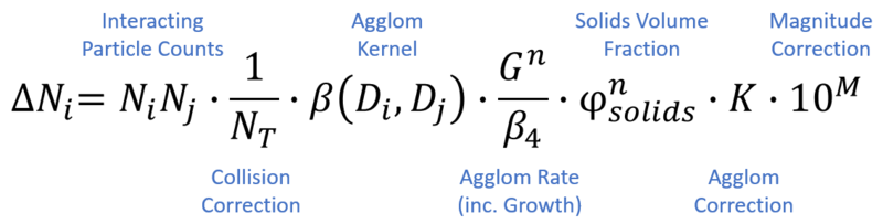
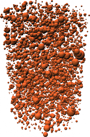
None of the literature attempts to characterize just where the transition between these two systems may lie, but state that there is no particular demarcation between the two. Both forms have been implemented and are available through the tag Agglom.Collision.Type. Note that [math]\displaystyle{ N_t }[/math] is proportional to solids content - as such, a power term on solids volume fraction is provided to account for effect of solids concentration on agglomeration, if required.

Here is 1%, 6% and 23% by volume of solids, at 23% by volume solids, which is typical for precipitation tanks, it appears that the system is restricted-in-space rather than free-in-space. Another example at 200, 400 and 800g/L is presented here (YouTube link).

1%	6%	23%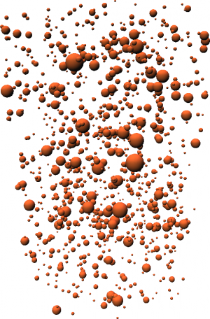

Agglomeration Cutoff

Generally, agglomeration of larger particles either does not occur, or occurs at a rate much slower than for smaller particles. In some cases, the size interaction predicted by the agglomeration kernel does not fall off quickly enough with increasing particle size. To adjust for this, there is an option that allows user to select the cutoff size for agglomeration. If selected, particles larger than the user-specified Agglom.Cutoff.Size will not agglomerate (kernel value is set to zero).

Some kernel forms allow for a steeper fall off in agglomeration rate so that the agglomeration cutoff can effectively be built into the kernel directly and the agglomeration cutoff limit may not be required.

Agglomeration cut off calculation correction in SysCAD 138: In projects which do use the agglomeration cutoff, there has been some adjustment to the calculation method and those project should be re-tuned as below.

• Any Probal projects using agglomeration cutoff should be retuned with Agglom.UseCorrectedCutoff selected. (Old projects will retain the original results until this is done)
• This will give a correct size distribution curve and also ensures that the model gives the same results as Dynamic projects with the same parameters when run to steady state.
• If not using agglomeration cutoff, no action is necessary

Attrition

The PSD models have no direct implementation of attrition processes, however it is straightforward to use other size changing models to implement this.

Suppose we observe quantities of fines being generated in a cyclone and we want to include this in the model. We can use the Crusher2 model as follows, adding it to the circuit following the cyclone overflow:

We use the Select/Break method for the crusher2 model: this allows us to select some fraction of particles from each bin and specify which bins they end up after we Break them.

In this simple example, we completely "break" some small fraction of particles in each bin and move them to fines.

• Note that the fines bin is 1.0-1.3 microns, particles in the bin 0-1 micron are coalesced and moved to this bin in the precipitator model.

• We specify the selection (.0001%) and move 100% of these broken particles to bin 1

• This isn't an exact model of attrition, but it is a good approximation for generating small mass fractions (though possibly large numbers) of fine particles.

• A more exact model would conserve total particle numbers in the non-fines bins.

• This could be implemented by moving some of the breakage to the next smaller bin, and some to the fine bin, with the proportions calculated to conserve mass and non-fines numbers.

• Custom calculations like these can be implemented in PGM code in a general controller. (Please see Example PGM File)

• Another approach is to manipulate the PSD curve directly using the Modify SzDist.Action

Area Correction

Nonspherical particles can have higher surface area for a given mass. This parameter can be adjusted to correct the surface area available for nucleation and growth due to nonsphericity.

Each of these "particles" has the same volume (and hence mass) but compared to the "spherical" particle on the right, the others have 16% and 58% greater area.

Using the Full PSD model

Discussion Page Alumina Precipitation and Classification with PSD

Most of the functionality in the existing Precipitator3 model carries over into the full PSD version - so the information in the first two tabs in the access window is still applicable. Growth is defined by the same equations as used in the non PSD part of the model, and this is set on the Precip Tab Page.

The new functionality is available on a separate tab page, titled PSD. There are a number of options and parameters that relate to PSD that the user can change, and there are various results specific to PSD that are displayed on this page. These fields are described in the PSD Tab Page.

Notes on parameters:

1. There are options Growth.On, Agglomeration.On and Nucleation.On which allow for turning the individual mechanisms on and off. A tank can be put into Growth Only mode by turning off Agglomeration.
2. For tuning, there are rate correction factors Growth.Rate.Correction, Agglom.Rate.Correction and Nucl.Rate.Correction.
3. SeedPSD: If no THA solids are found in the incoming stream, then a small quantity will be generated. This is sufficient to seed a tank, and in subsequent iterations, the recycles will take over and provide the necessary solids.
4. See PSD Tab Page for a full description of all fields, including results.

Note that the nucleation yield is generally negligible compared to the growth yield, though nucleation is necessary to spawn new particles that eventually grow and become seed sites for growth.

Summary of Agglomeration forms and units

Particle numbers in SysCAD are represented as #/kg slurry, while for agglomeration calculations we work with #/m^3 slurry - to convert from #/kg to #/m^3, multiply by the slurry density.

In volume terms, the discretized equations are

[math]\displaystyle{ \dot N_i = \sum_j \beta_{ij} N_i N_j }[/math]

and

[math]\displaystyle{ \dot N_i = \sum_j \beta_{ij} N_i N_j/N_t }[/math]

for the FIS and RIS forms. We also separate the kernel [math]\displaystyle{ \beta_{ij}=\beta_p \beta_{gij} }[/math] into process related and geometric components - the latter are fixed and can be precalculated, while the former will change as process conditions vary, but is the same for each kernel term. The units for various methods are summarized here.

The agglomeration rate reported in the access window is the process part of the kernel term - for the size independent kernel this is just the same as </beta> since there is no geometric contribution.

Rate Constants for Agglomeration

In general, determining appropriate rate constants is a matter of tuning. The supplied default constants are suitable for the RIS, size independent kernel (default) and will be unlikely to work for other settings. Note that for the RIS implementation, there is an additional term [math]\displaystyle{ 1/N_t }[/math] in the agglomeration calculation. Since the number of particles (per cubic meter) is of the order of [math]\displaystyle{ 10^{12} }[/math], our rate "constants" will be very different.

Because different kernel forms and agglomeration calculations will have different interpretations of the units of the rate constant, we do not provide these: using this model you should experiment with values of the constants to determine a suitable range,

If the overall rate constant is too high, then all particles will be "agglomerated away" ending up with a distribution having low surface area and little growth. If it is too low, then there will be no agglomeration effects. There will be a fairly narrow window in overall rate over which effective agglomeration will take place.

For the example distributed with SysCAD (Full PSD Precipitation Circuit) we find behaviour as follows as we vary the overall agglomeration rate:

The upper and lower curves show the product d50 and total production. As we increase the agglom factor, the product d50 increases and the production drops off. There is some initial increase in production, but this is related to the temperature and hence yield increasing - for low values, large amounts of fine seed is recirculated since growth is not providing a lot of coarse particles. You find the recirculation rates are three or four times the incoming liquor flow.

The key point: Increasing agglomeration decreases total yield since it decreases the surface area available for growth

So for low values of the factor you get high total production and large numbers of fine particles. For high values you get low production and small numbers of coarse particles, since there is little surface area for yield. A given plant will operate somewhere in this range, and you can tune the agglomeration rate to match observed data.

Suppose quality tests have shown that 10% of particles in the product are out of spec (e.g. below 45 microns) Assuming the rest of the model is perfectly tuned, then an agglomeration constant of 0.1 would lead to 23% of the particles below 40 micron, while a constant of 1.0 will lead to just 8% being out of spec. The overall constant is probably somewhere in this range and can be tuned accordingly.

NOTE: You should follow these general guidelines in tuning to determine suitable values for the agglomeration parameters - and these will be different for the different kernels and agglomeration methods.

Adjusting the Full PSD Precipitation parameters

There are hundreds of papers on precipitation rate processes and the various parameters that influence the different mechanisms. For example, the type of agitation or energy dissipation strongly influence the agglomeration rate.

Since there are many possible tank configurations, the SysCAD PSD model provides only the basic framework. The user can account for additional effects by adjusting the core model parameters. In particular, the rate correction parameter is useful in this regard.

Adjustment for other parameters

So for example if we want to correct for tank agitation rate, and experimental data suggests that the rate has a form

[math]\displaystyle{ r = 0.3 + 0.00124 f }[/math]

where [math]\displaystyle{ f }[/math] is the impeller rate.

A simple example of how to implement this to make the adjustment in the model is shown below: the PGM logic will be added via the General Controller.

TextLabel(,"Tank Parmeters")
REAL ImpellerRate*("pS", "rpm")<0,200><<35>>
REAL AggRateCorrection@
...

Sub InitialiseSolution()
  AggRateCorrection = 0.3 + 0.00124 * ImpellerRate^1.4
  ["PC_001.Agglom.Rate.Correction"] = AggRateCorrection
  ...
End Sub

An extension of the above example to include calculation for display of overall Yield and Production is shown below:

TextLabel(,"Tank Parmeters") REAL ImpellerRate*("pS", "rpm")<0,200><<35>> REAL AggRateCorrection@ TextLabel(,"Yield Calculations") REAL MW_Al2O3,MW_Na2CO3 REAL Production@("Qm", "t/d") REAL Yield@("Conc", "g/L") Sub InitialiseSolution() MW_Al2O3 = MW("Al2O3(s)") MW_Na2CO3 = MW("Na2CO3(aq)") AggRateCorrection = 0.3 + 0.00124 * ImpellerRate^1.4 ["PC_001.Agglom.Rate.Correction"] = AggRateCorrection EndSub ;P_012 is product stream and P_011 is pregnant liquor feed stream Production = ["P_012.Qo.SQm (t/d)"] Yield = Production / ["P_011.Qv (kL/d)"] *1000. * MW_Al2O3/MW_Na2CO3 $END OF FILE

Implementing new correlations

For growth rate you can use the FixedRate method together with your own growth rate correlation calculated in PGM code. Suppose we want to implement the Ilievski correlation, again using some PGM logic in a General Controller model:

[math]\displaystyle{ G = k_H \cfrac{C/A^* - .608}{C/A -.608} }[/math]

We can define a function in the PGM code, so we can reuse it if we want to have the correlation available for a number of tanks:

TextLabel(,"Ilievski Growth Rate") REAL K_H*<<0.1>> REAL A@("Conc", "g/L"){Comment("@25C")} REAL ASat@("Conc", "g/L"){Comment("@T")} REAL C@("Conc", "g/L"){Comment("@25C")} REAL G@("Ldt", "um/h") Function IlievskiRate(REAL A, REAL ASat, REAL C, REAL kH) Double tmp1 tmp1 = C-0.608*A If (tmp1 <= 0 or ASat <=0) return 0.0 Endif return Range(0.0, kH*A/ASat*(C - 0.608*ASat)/tmp1, 20.0) EndFunct ;Setting the GrowthRate ASat = ["PC_001.QProd.Props.A_Saturation (g/L)"] A = ["PC_001.QProd.Props.AluminaConc (g/L)"] C = ["PC_001.QProd.Props.CausticConc (g/L)"] G = IlievskiRate(A, ASat, C, K_H) ["PC_001.FixedGrowthRate (um/h)"] = G ;... $ END OF FILE

The GC now has fields to enter the Ilievski correlation K, as well as displaying the tank parameters that are used in the correlation. When the model is run, the calculated value of G is copied to the tank FixedGrowthRate field, and used in subsequent calculations:

NOTES:

• We only need to set the Agglomeration Rate correction once (on initialize) since this doesn't change with tank conditions
• However since the tank conditions change as we solve - the alumina and caustic concentrations will vary - then we need to recalculate the rate at each iteration
• When you are implementing your own correlations you are responsible for making sure that the calculation can be done and that resulting numbers are sensible. So it is vital to check that you don't have divide by zeros, and that the final result lies in a proper range.
• The Range function is useful here.

Sample Circuit

This example shows the essentials of a precipitation circuit, using the full PSD model. This project is distributed with SysCAD and is located with the other Alumina example projects.

Pregnant liquor is introduced to the first tank in the row, along with fine seed. There is also allowance for the possibility of introducing 'charge seed though this is not necessary for the new model. The first three tanks act as agglomeration tanks, and coalesce the fine seed.

Coarse seed is introduced in the fourth tank, and the remainder of the row tanks are growth tanks.

The pumpoff from the final tank is sent to a cyclone, which splits it into fine and coarse streams. The fines are deliquored and passed back to the first tank along with the pregnant liquor. The coarse cut cyclone underflow is split - some fraction is deliquored and sent back as coarse seed to the first growth tank, and the remainder is available as actual product.

We can for example track the PSD down the row

This is not particularly enlightening, but we can track the d50 cuts or the surface area:

A sample Excel SysCAD_TagTable() report is included with the example, and used to generate the data for these plots.

NOTES

In reality circuits are far more complex, with multiple cyclones, filters, classifiers and various splits to different points in the precipitation row. However this example captures the essential features of a precipitation circuit.

The circuit is self seeding - if there are no PSD solids (THA) present in a tank, then trace amounts of fine solids will be added. This is necessary since the pregnant liquor may contain no solids, and in theory nucleation and growth only occur on existing particles. Even a miniscule amount of solids will increase through the row and by feeding back to the start of the circuit, eventually build up to equilibrium conditions.

In other implementations (and in actual startup of a real refinery), some seed is required to charge the circuit. A refinery startup will actually involve trucking or shipping in several thousand tonnes of alumina from another refinery, then charging a number of the tanks to say 100gpl solids during commissioning.

The Charge Seed stream in this flowsheet is thus not necessary (and has no flow in the example), though could be used in a full dynamic model to simulate the startup transient conditions.

Setting up the PSD Definition

The present implementation requires geometrically spaced bins, with a size ratio of [math]\displaystyle{ \sqrt[3]{2} }[/math]. The easiest way to specify this sieve series is to use the Q option, with a Q-value of 1.0

Refer to Size Configuration for more detail on sieve series construction.

The Alumina3 models use a particular form for THA (trihydrate alumina) as a species - Al[OH]3(s) - and this should be selected in the Size Distribution tab:

• Mutiple sieve series can be used, but the first one must satisfy these conditions. Other sieve series should be added after this one. For example if you have sizer data for non geometrically spaced bins that you want to convert, add the new sieve series following the first one.

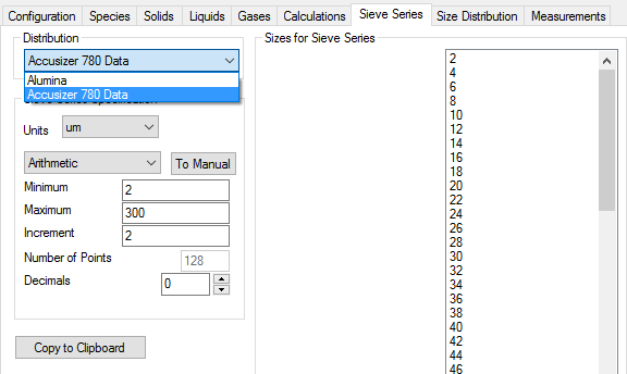
NOTE: The new Distribution needs to be defined in the Size Distribution tab first,
then it can be selected on the Sieve Series tab.

Sensitivity to Bin numbers

In all the Alumina models we have examined, the particles range in sizes from 1 micron to 1000 micron, however 500 micron is a more typical upper limit.

We examine the results of the model of a full PSD circuit with two different ranges: 4 micron to 406 micron (21 bins) and 1 micron to 512 micron (28 bins). The key parameter is product quality - the results below are for the product.

With Agglomeration                        Without Agglomeration
    28 bins            21 bins             28 bins         21 bins
----------------------------------------------------------------------
d50  203.8615321       192.9754881         164.8114539     159.1629558
d80  154.744547        144.6053441         106.4823075     107.4396741
SAM  0.017167115       0.018641902         0.030099571     0.028748622
SAL  41.53447717       45.1024256          72.82220833     69.55330719

References

[1] M.J. Hounslow, R.L. Ryall, V.R. Marshall (1988) "A discretized population balance for nucleation, growth and aggregation" AIChE. J, 11

[2] C. Misra (1970) "The precipitation of bayer aluminium trihydroxide" PhD Thesis. University of Queensland

[3] I. Livk, D. Ilievski (2007) "A macroscopic agglomeration kernel model for gibbsite precipitation in turbulent and laminar flows" Chemical Engineering Science 62

[4] D.N. Seneviratne, H. Peng, A.R. Gillespie, J. Vaughan (2018) "An investigation of Bayer desilication product agglomeration mechanisms by kernel function population balance modelling" Alumina2018: the 11th AQW International Conference

[5] R. Peña, C.L. Burcham, D.J. Jarmer, D. Ramkrishna, Z.K. Nagy (2017) "Modeling and optimization of spherical agglomeration in suspension through a coupled population balance model" Chemical Engineering Science 167

[6] I. Golovin, G. Strenzke, R. Dürr, S. Palis, A. Bück, E. Tsotsas, A. Kienle (2018) "Parameter Identification For Continuous Fluidized Bed Spray Agglomeration" Processes 2018

[7] W.J. Crama, J. Visser (1994) "Modelling and computer simulation of alumina trihydrate precipitation" Light Metals 1994

[8] H. Eisenschmidt, M. Soumaya, N. Bajcinca, S. Le Borne, K. Sundmacher (2017) "Estimation of aggregation kernels based on Laurent polynomial approximation" Computers & Chemical Engineering 103

[9] V.G. Levich (1954) "The Theory of Coagulation of Colloids in Turbulent Liquid Stream" Dokl. Akad. Nauk SSSR 1954, Vol.99

[10] D. Green, R. Perry (2008) "Modelling and Simulation of Granulation Processes" Perry's Chemical Engineers' Handbook 8th Ed. 21-143

[11] R. David, A. Paulaime, F. Espitalier, L. Rouleau (2003) "Modelling of multiple-mechanism agglomeration in a crystallization process" Powder Technology, Elsevier, 2003, 130 (1-3, SI), pp.338-344

[12] R. David, F. Espitalier, A. Cameirão, L. Rouleau (2003) "Developments in the Understanding and Modeling of the Agglomeration of Suspended Crystals in Crystallization from Solutions" KONA No.21