Crusher 2 Model Theory
Navigation: Models ➔ Size Distribution Models ➔ Crusher2 ➔ Model Theory
| Crusher2 | Crusher 2 Model Theory |
|---|
Model Theory - Fixed Partition Method
The user defines a fixed size distribution (partition) as the product from the Crusher.
The model will produce the user defined size distribution even if this would result in the crusher producing a coarser product than feed. This is best demonstrated using an example:
|
Size' Range' (mm) |
Feed Fraction (%) |
Required Discharge |
| +10.00 | 20 | 15 |
| +1.70 | 10 | 15 |
| +0.85 | 15 | 20 |
| +0.50 | 15 | 10 |
| +0.10 | 20 | 10 |
| +0.01 | 15 | 10 |
| -0.01 | 5 | 20 |
| (sum) | (100) | (100) |
In the above example, there is enough material in the +10.0mm and +1.7mm feed size ranges to meet the required discharge product size distribution. For the +0.85mm size range only 15% is available where 20% is requested.
Model Theory - Whiten Crusher Method
This is an empirical model incorporating breakage and classification, based on the key parameter [math]\displaystyle{ T_{10} }[/math] for breakage, and parameters [math]\displaystyle{ K_1, K_2 }[/math] and [math]\displaystyle{ K_3 }[/math] for classification.
The form of the Whiten classification function is:
- [math]\displaystyle{ C(x) = 1-\left(\cfrac{K_2-x}{K_2-K_1}\right)^{K_3}, \qquad K_1 \lt x \lt K_2 }[/math]
Where the parameters K1, K2 and K3 can be entered directly or calculated from equipment variables and operating conditions.
The actual breakage function is determined as a spline fit to test data which is specified as well.
If the key parameters are calculated, the following correlations are used:
- K1 = A0 + A1*CSS - A2*TPH + A3*F80 + A4*LLEN
- K2 = B0 + B1*CSS + B2*TPH + B3*F80 - B4*LHR + B5*ET
- T10 = D0 - D1*CSS + D2*TPH - D3*F80
- where
- CSS = Closed Side Setting (mm)
- TPH = Throughput (dry t/h)
- F80 = 80% passing size of Feed (mm)
- LLEN = Length of face of mantle liner (mm)
- LHR = Liner age (hours)
- ET = Eccentric Throw (mm)
- A0 to A4 are parameters for K1, obtained from data fitting.
- B0 to B5 are parameters for K2, obtained from data fitting.
- D0 to D3 are parameters for T10, obtained from data fitting.
Notes:
- These are linear offsets to base values which depend on the operating conditions and crusher configuration. See MCC for further discussion.
- The parameters A0, B0 correspond to base values of K1, K2
- The parameters A1, A2, A3, A4, B1.. B5 are hidden and by default set to zero. Un-hide these fields if you need to adjust the K values based on operating conditions and crusher configuration.
- So K1=A0 and K2=B0 if other parameters are not set.
Ore Specific Breakage
The ore properties are given as a table (MCC Table 6.1, General appearance function for crusher model)
This data is determined by various ore tests. The default values are those from MCC.
A second table is provided for ore specific comminution energy, Ecs. This gives the size specific energy needed to achieve a particular degree of breakage.
Reference
Napier-Munn et al "Mineral Comminution Circuits - Their Operation and Optimisation (MCC)", Chapter 6
Model Theory - Selection/Breakage Method
In the subsequent discussion we use the following notation, loosely following that of Taveres[1] for discrete bin PSD modelling.
The SysCAD PSD model is based on a user supplied sieve series, with sizes [math]\displaystyle{ D_0, \,D_1\dots D_N }[/math] which form N bins, with bin k containing particles in the size range [math]\displaystyle{ D_{k-1}\leq x \lt D_k }[/math]. Each bin has a characteristic size [math]\displaystyle{ d_k }[/math], which is typically the geometric mean of the upper and lower sizes, though this can be modified by a user supplied correction.
The new comminution model implements a number of open literature correlations for selection and breakage. The overall breakage function is composed of both a selection function (breakage probability) and a breakage distribution (fragment size distribution).
Breakage Probability Selection Functions
In the following equations [math]\displaystyle{ S_i }[/math] is the probability that a particle in bin i breaks.
Vogel Selection Function
- [math]\displaystyle{ S_i = 1-e^{-f_{mat} \; d_i \, k(W_{m,kin} \;\; -W_{m,min} \;\;)} }[/math]
- where:
- fMat = Material Parameter that characterises the resistance of particulate material against fracture in impact comminution.
- Wm_kin = Mass-specific kinetic impact energy.
- Wm_min = Mass-specific threshold energy for particle breakage, i.e. the specific energy which a particle can take up without fracture.
Note that in the SysCAD model, a size independent specific energy is specified, i.e. [math]\displaystyle{ x\times W_{m,min} }[/math]
- k = Number of impact events.
Reference
Vogel-Peukert, Breakage Behaviour of Different Materials - Construction of a Mastercurve for Breakage Probability, Powder Technology, 2003.
Austin Selection Function
- [math]\displaystyle{ S_i = S_1 \left( \cfrac{d_i}{d_1} \right)^\alpha }[/math]
- where:
- S1 = Material Parameter. 0 <= S1 <= 1
- [math]\displaystyle{ \alpha }[/math] = Parameter. 0 <= [math]\displaystyle{ \alpha }[/math] <= 1
- d1 = Minimum particle size. 0 <= d1 <= dmax
- dmax = Maximum particle size in the feed stream
Reference
Austin L.G. et al, A Rapid Computational Procedure For Unsteady-State Ball Mill Circuit Simulation, SME-AIME, 1984.
Breakage function for discrete bins
The Breakage function is actually a continuous function.
- The Reid and Stewart form (basically a double Schumann equation) is
- [math]\displaystyle{ B(X) = \Phi\left(\cfrac{X}{X_0}\right)^\gamma+(1-\Phi)\left(\cfrac{X}{X_0}\right)^\beta }[/math]
- This calculates the fraction of particles of size [math]\displaystyle{ X_0 }[/math] that will end up smaller than size X after breakage.
In the discrete form, we start with the following cumulative breakage curves.
Here [math]\displaystyle{ B_{ji} }[/math] = Fraction of particles from a bin of characteristic size i breaking below size j
Reid-Stewart form (Perry)
- [math]\displaystyle{ B_{ji} = \Phi\left(\cfrac{D_j}{d_i}\right)^\gamma+(1-\Phi)\left(\cfrac{D_{j}}{d_i}\right)^\beta }[/math]
- where:
- [math]\displaystyle{ \Phi }[/math] = Experimentally determined material parameter.
- [math]\displaystyle{ \gamma }[/math] = Experimentally determined material parameter.
- [math]\displaystyle{ \beta }[/math] = Experimentally determined material parameter.
Reference
Perry et al Perry's Chemical Engineers' Handbook 6th or 7th Edition, McGraw-Hill 1984.
Austin Breakage Function
- [math]\displaystyle{ B_{ji} = \Phi\left(\cfrac{D_j}{d_i}\right)^\gamma+(1-\Phi)\left(\cfrac{D_{j+1}}{d_i}\right)^\beta }[/math]
- where the parameters are the same as for the Reid-Steward form above.
- The Austin form allows for complete breakage of all selected particles in a bin since
- [math]\displaystyle{ \frac{D_{j+1}}{d_j}\gt 1 }[/math] will force the cumulative function to be greater than 1 (and thus set to 1 for breakage to the same bin).
Vogel Breakage Function
- [math]\displaystyle{ B_{ji} = \cfrac12\left(\cfrac {D_j}{d_i}\right)^q\left[1+\tanh\cfrac{D_j-x'}{x'}\right] }[/math]
Tavares Breakage Function
- This implementation uses a single constant [math]\displaystyle{ t_{10} }[/math] supplied as a parameter
- [math]\displaystyle{ B_{ji} = 1-(1-t_{10i}) ^{\left[\cfrac9{d_i/D_j-1 \;}\right]^\alpha} }[/math]
- where
- [math]\displaystyle{ \alpha }[/math] = Material Parameter based on experimental data.
- t10 = Material Parameter
Reference
Tavares Optimum Routes for Particle Breakage by Impact, Powder Technology 142, 2004.
Logarithmic form
- [math]\displaystyle{ B_{ji} = A\ln\cfrac{D_j}{d_i}+1 }[/math]
- where
- A = Material Parameter
User Weibull form
- [math]\displaystyle{ B_{ji} = 1-\exp \left[-\left(\cfrac{x - x_u}{x^*-x_u}\right)^n \right] }[/math]
- where
- [math]\displaystyle{ x = \cfrac{D_j}{d_i} }[/math]
- n = User Parameter. n>0
- xu = User Parameter
- x* = User Parameter: x* > xu
Notes
- For all these distributions, the fractional breakage from bin i into bin j is then just the difference of the cumulative breakages between the upper size and lower size.
- The Reid, Taveres, Log and Weibull distributions are scale invariant and only depend on the ratio of mother to daughter particle size.
- The Vogel breakage distribution depends on the impact velocity
Multiple Impact Events
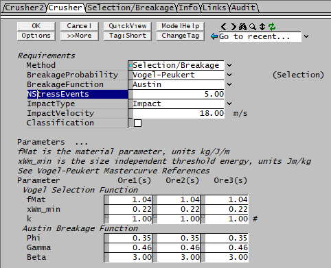
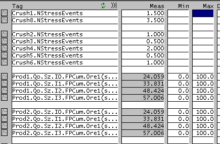
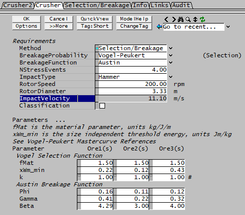
In some crushing operations, material is subject to multiple impact events. The parameter NStressEvents is used to model this.
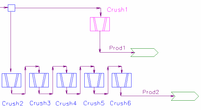
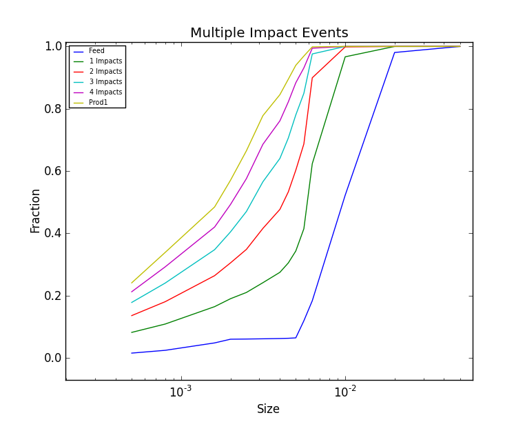
With N multiple impact events, the results are identical to having N individual crusher units with the same parameters and one impact event:
Following the PSD distribution through the multiple events:
Fractional Impact Events
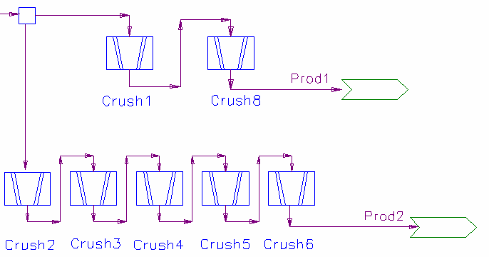
The number of stress events need not be an integer. It is possible to have 1.5 stress events, which would correspond to a situation where some of the feed undergoes two impacts.
The result of having two crushers with 2.5 impact events is the same as having five crushers with a single impact event or any other combination adding up to the same total:
Impact Velocity
The selection (and some of the breakage) models involve a velocity or specific energy which is user supplied.
- For an impact mill, this is just the impact velocity;
- For a hammer mill, it is calculated from rotation speed and diameter.
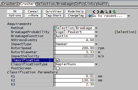
Classification
When internal classification is turned on, additional parameters are available for the classification function
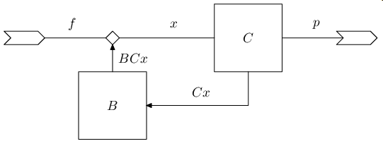
With internal classification, particles of larger sized are retained in the mill; the overall internal flow of material can be represented as follows.
The model allows user entry for all the parameters (Selection, Breakage and Classification). If there are multiple ores, data is only displayed for a single ore, and the user can select which ore to display.
Using this representation, we can model other configurations. A simple closed-circuit milling system (see example image on Wikipedia) has the following transfer function:
Model Theory - Test Data
The user enters the size fractions of the Crusher Feed and Product from test work. The model calculates a pseudo selection and breakage function from the entered test data to "estimate" the crusher output from a given crusher feed distribution.
Algorithm
Assume you have test data consisting of feed size fractions F and product fractions P.
- We define the amount of material AVALIABLE of a size fraction i to be broken to the next size fraction to be:
- [math]\displaystyle{ \mathbf{\mathrm { A_i = F_i + A_{i+1}\times B_{i+1}}} }[/math]
- where
- F_i is the feed in for this size fraction i
- F_{i+1} is feed in for the next largest size fraction i+1
- Define EXTENT of size fraction retained as [math]\displaystyle{ \mathbf{\mathrm { E_i = P_i/A_i }} }[/math]
- Define BREAKAGE from one size fraction to the next as [math]\displaystyle{ \mathbf{\mathrm { B_i = 1 - E_i}} }[/math]
- From the test data we can calculate the A(i) data and hence B(i) and E(i)
- Then we can "estimate" the new products as
- [math]\displaystyle{ \mathbf{\mathrm {\boldsymbol{P}_i^{est} = \left(F_{i+1}^{act}\times B_{i+1} + F_i^{act}\right)\times E_i}} }[/math]
- i.e. Estimated Product at Size = [ Actual Feed at previous size*breakage at previous size + Actual Feed at Size ]*[ 1 - Breakage at size ]
- From the test data, starting at the largest size fraction it determines the fraction that reports to the next size down and then adds this to the feed of that, determines the fraction that reports to the next size down and so on.
- Essentially the broken amount from the previous size fraction is assumed to report to the next size fraction for breaking.
Example
Size (mm) Fi
Feed (kg)Pi
Product (kg)Ai
Amount of material available
for breakdown to next size (kg)Bi
Breakage (kg)Ei
Retained (kg)100 10 8 10 2/10 8/10 80 8 6 8+2/10*10 = 10 4/10 6/10 60 6 6 6+4/10*10 = 10 4/10 6/10 40 5 7 5+4/10*10 = 9 2/9 7/9 20 4 6 4+2/9*9 = 6 1/6 1


