Python Example - Optimisation
Navigation: User Guide ➔ COM Automation ➔ Python Automation ➔ Example - Optimisation
Related Links: Example Project - ChemApp with Python Optimisation
Overview
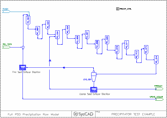
This example demonstrates using a number of tools to tune a steady state model (SysCAD project) based on data. This uses the Demo Precip Circuit in the distributed examples.
We are provided with a product size distribution (for example from plant data) and we want to adjust some key parameters to tune the model to this data.
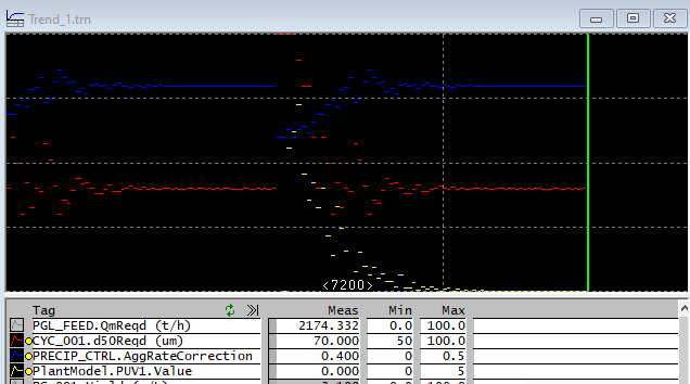
The two parameters we will adjust are the Agglomeration Rate and Cyclone Cut Size. Add the latter to the Trend Window so you can watch how these change as the optimisation proceeds.
In some ways this is an example of curve fitting - which is just another optimization problem. The curve fitting problem - find the "best fit" of a function with a small number of parameters to a set of data points, which means minimising the difference between the given data and the fit in some norm. Usually curve fitting involves evaluating a simple function to generate the fit. In this case, we generate the fit by running SysCAD while varying a small number of parameters.
Calculating the Objective Error
A key concept of optimisation is an objective function which is a target we want to minimise. In this case the target is to minimise the difference between the desired PSD and one our model calculates. We can calculate the objective function either in a PGM or in python - in an earlier version of this example we showed this in PGM, but we will now do the calculation in python. (A PGM listing is here, where the error is calculated and then fetched to the optimiser as a single value)
- We use the SysCAD COM Interface Class from the introductory notes
- A more common target is minimisation of some "cost" associated with a particular configuration, or maximisation of "revenue". This would take into account total production (revenue) minus costs (for energy and raw materials).
- In this example we calculate the objective function in python by fetching the PSD distribution using COM.
target = np.array([2.97869e-05, 3.93492e-05, 5.69551e-05, 8.58349e-05, 0.00013228, 0.00020766,
    0.00033343, 0.00055317, 0.00096398, 0.0018091, 0.0037611, 0.0087440, 0.022172,
    0.058889, 0.159535, 0.440231, 1.256861, 3.695465, 10.19094, 21.37749, 27.96972,
    21.47619, 9.873492, 2.837389, 0.542968, 0.073854, 0.0080610])

        psdist = np.array(sc.getTags(PSDTags))
        err = np.linalg.norm(psdist/target-1)
Python Optimisation
We will use the scipy optimisation module as well as numpy, so we import those. (These are part of the Anaconda distribution, otherwise pip install numpy/scipy)
import numpy as np
import scipy.optimize as spo
The scipy.optimize module has a function fmin, which is the the Nelder-Mead downhill simplex algorithm
>>> help(spo.fmin)
Help on function fmin in module scipy.optimize.optimize:
fmin(func, x0, args=(), xtol=0.0001, ftol=0.0001, maxiter=None, maxfun=None, full_output=0, disp=1, retall=0, callback=None, initial_simplex=None)
   Minimize a function using the downhill simplex algorithm.
   This algorithm only uses function values, not derivatives or second
   derivatives.
This takes a function (in python speak callable) (which is the objective function we want to minimise) and a starting point, plus a number of optional further parameters.
The callable func takes a single array argument func([x1, x2...]) , and evaluates the objective at these values, returning this result. In our case here, evaluation of the objective function means running SysCAD with the tags we want to adjust for opimisation set to these values, and return our calculated error. We have a list of optimising tag strings, and also need to fetch the outlet size distribution:
optTags =  ["PRECIP_CTRL.AggRateCorrection",  "CYC_001.d50Reqd (um)"]
PSDTags = ["P_011.Qo.Sz.I%d.FP.Al[OH]3(s) (%%)" % i for i in range(1, 28)]
Then our objective function is just
    def f(z):
        sc.setTags(optTags, z)
        sc.run()
        psdist = np.array(sc.getTags(PSDTags))
        err = np.linalg.norm(psdist/target-1)
        sc["PlantModel.PUV1.Value"]=err        ## We store this back in SysCAD so we can plot the error in the trend window
        return err
Having defined this, then we just make a call to fmin with some suitable starting values (in the code, just fetch the existing tags)
res = spo.fmin(f, ystart)
Thats all there is to it!
The desired PSD distribution was actually determined by running the model with agglomeration correction 0.4 and cut size 70 microns, and these valued are recovered by the optimization.
Be sure to call doClose() after finishing to clean up COM objects, otherwise you end up with zombie SysCAD instances. (If strange things are happening use Process Explorer or Task Manager to remove these)
Optimization terminated successfully.
         Current function value: 0.000053
         Iterations: 39
         Function evaluations: 74
[ 0.40000361 69.99949443]
#! python3 -i
## Optimisation with COM and python.

import syscadif
import numpy as np
import scipy.optimize as spo

ScdPrj = r'C:\SysCAD139\Examples\10 Alumina\PSD Precipitation Circuit Example.spf\Project.spj'
optTags =  ["PRECIP_CTRL.AggRateCorrection",  "CYC_001.d50Reqd (um)"]
PSDTags = ["P_011.Qo.Sz.I%d.FP.Al[OH]3(s) (%%)" % i for i in range(1, 28)]

target = np.array([2.97869e-05, 3.93492e-05, 5.69551e-05, 8.58349e-05, 0.00013228, 0.00020766,
0.00033343, 0.00055317, 0.00096398, 0.0018091, 0.0037611, 0.0087440, 0.022172,
0.058889, 0.159535, 0.440231, 1.256861, 3.695465, 10.19094, 21.37749, 27.96972,
21.47619, 9.873492, 2.837389, 0.542968, 0.073854, 0.0080610])

sc = syscadif.SysCADCom()
sc.OpenProject(ScdPrj)

def main():
    ## start from saved solution
    ystart = np.array(sc.getTags(optTags))
    print (ystart)

    def f(z):
        sc.setTags(optTags, z)
        sc.run()
        psdist = np.array(sc.getTags(PSDTags))
        err = np.linalg.norm(psdist/target-1)
        sc["PlantModel.PUV1.Value"]=err   ## We store this back in SysCAD so we can plot the error in the trend window
        return err

    res = spo.fmin(f, ystart, xtol=.001, ftol=.05)
    print (res)

main()
input('Enter to finish')
sc.Close()
|
Remarks
- You could also do optimisation based on tuning external parameters instead of SysCAD tags, for example in PHREEQC.
- The objective function could also be calculated in PGM, e.g.:
;--- variable declarations ---
PageLabel(Precip)
    TextLabel(,"Recycle mass flows")
    REAL 	FS_SolidRecovery*("Frac", "%")
    REAL 	FS_Solids_Moisture*("Frac", "%")
    REAL 	CS_SolidRecovery*("Frac", "%")
    REAL 	CS_Solids_Moisture*("Frac", "%")
    TextLabel(,"Global Agglomeration correction")
    Long	i, NumberofTanks*<<14>>
    REAL 	AggRateCorrection*
    TextLabel(,"Yield Calculations")
    REAL 	Production@("Qm", "t/d")
    REAL 	Yield@("Conc", "g/L")
    REAL 	ProductD50@("L", "um")
    TextLabel(,"Check SysCAD Version", "Function IntStr0 available in SysCAD9.3 Build136.19015")
    Checkbox BuildOK@

;; Constant Array with desired product size distribution
Array z = {2.97869e-05, 3.93492e-05, 5.69551e-05, 8.58349e-05, 0.00013228, 0.00020766,
0.00033343, 0.00055317, 0.00096398, 0.0018091, 0.0037611, 0.0087440, 0.022172,
0.058889, 0.159535, 0.440231, 1.256861, 3.695465, 10.19094, 21.37749, 27.96972,
21.47619, 9.873492, 2.837389, 0.542968, 0.073854, 0.0080610 }

;; Work array
Array x
PageLabel(Analysis)
TextLabel(, "Error difference between product PSD and desired PSD")
real PSDError@

Sub InitialiseSolution()
    ["X_003.Separ.SolidsToUFReqd (%)"]    = FS_SolidRecovery
    ["X_003.Separ.UFSolidFracReqd (%)"] = 100 - FS_Solids_Moisture
    ["X_001.Separ.SolidsToUFReqd (%)"]    = CS_SolidRecovery
    ["X_001.Separ.UFSolidFracReqd (%)"] = 100 - CS_Solids_Moisture

    i = 1
    While i <= NumberofTanks
    	[Concatenate("PC_", IntStr0(i, 3), ".Agglom.Rate.Correction")] = AggRateCorrection
    	i = i + 1
    EndWhile
    x.SetLen(27)
EndSub

    Production =  ["P_011.Qo.SQm (t/d)"]
    Yield = Production/["P_012.Qv (kL/d)"]*1000.*102./156.
    ProductD50 = ["P_011.Qo.Sz.d50.Al[OH]3(s) (um)"]
    i = 1
    while (i<=27)
       x[i-1] = [Concatenate("P_011.Qo.Sz.I", IntToStr(i), ".FP.Al[OH]3(s) (%)")]
       i = i+1
    endwhile
    x.Div(z)
    x.Offset(-1)
    PSDError = x.inner(x)

$ ; --- end of file ---
|

