The printable version is no longer supported and may have rendering errors. Please update your browser bookmarks and please use the default browser print function instead.

Navigation: Models ➔ Size Distribution Models ➔ Hydrocyclone

General Description

This model is used to simulate either a single Hydrocyclone, or a cluster of Hydrocyclones.

The model is primarily designed to split solids based on size distribution data. Therefore, the feed should contain solids with size distribution information. The model will calculate the split of solids between the under and over flows based on the cut point (either calculated or defined) and the size distribution of the feed stream.

Using Size Distribution, the unit allows the user to define the cyclone in one of five ways:

Define the partition curve of the cyclone
Define the cut point, d₅₀, of the cyclone
Use the Krebs method to calculate the cut point
Use the Plitt method to calculate the cut point
Use the Nageswararao method to calculate the cut point

The first two options allow the user to set the cut point without any further knowledge of the cyclone. The next three options require the user to define the cyclone dimensions. These dimensions are then used to calculate the cut point and partition curve of the cyclone.

In the case of the Plitt and Nageswararao methods, the model will also calculate the liquid split between the over and under flows.

The Hydrocyclone may also act as a simple splitter, where the solids in the feed to the unit do not have any size distribution data. In this case the user must select Method = 'Simple (non PSD) Models' and set the solids and liquid split to the under and over flow streams.

Note: This unit cannot be used to model a gas cyclone.

Diagram

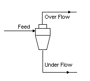
The diagram shows the default drawing of the Hydrocyclone, with all of the streams that are available for operation of the unit. The physical location of the streams connecting to the Hydrocyclone is unimportant. The user may connect the streams to any position on the unit.

Inputs and Outputs

Label	Required Optional	Input Output	Number of Connections		Description
Label	Required Optional	Input Output	Min	Max	Description
Feed	Required	In	1	20	The slurry feed to the Hydrocyclone
OverFlow	Required	Out	1	1	The over flow from the unit
UnderFlow	Required	Out	1	1	The under flow from the unit

Model Theory

The method of splitting the solids based on Size Distribution data is discussed below:

The model will simulate a Hydrocyclone using one of the five user defined methods - 'User Defined Curves', 'User d₅₀', 'Krebs Cyclone', 'Plitt Cyclone' and 'Nageswararao'. These are described below.
The 'User Defined Curves' method allows the user to define the fraction of material in each size interval that will report to the cyclone overflow.
The other methods use the d₅₀ value, either calculated or defined by the user, to determine the solids separation. The d₅₀ is defined as the particle size that has a 50% chance of reporting to either the cyclone underflow or overflow. The majority of the particles finer than this size will report to the overflow, while the majority of those coarser will report to the cyclone underflow.
The user may also define the number of Hydrocyclones in the cluster. The default value, and the minimum number, is 1. This allows the model to calculate the pressure drop across each cyclone by dividing the flow to the model by the number of cyclones in the cluster. This allows the user to model a number of Hydrocyclones with a single drawing.

The drawing to the left shows the dimensions that are used in the Plitt and Nageswararao models.

The Plitt model doesn't include the length of the cylindrical section as a parameter
The length [math]\displaystyle{ h }[/math] is the free vortex height, i.e. the distance from the underflow to the bottom of the vortex finder.
In the Nagasawarao model, the height [math]\displaystyle{ h }[/math] is implicitly calculated from the cone angle and the diameters assuming the free vortex occupies the conical section.

User Defined Curves (Efficiency Curve)

The user defines the Efficiency Curve of the cyclone by entering the fraction of material in each size interval that will report to the cyclone overflow. This will normally be the Actual efficiency curve, which takes into account the bypassing of fines to the underflow with the liquid.

An example of an Efficiency curve is shown to the left.

The user also defines the fraction of solids in the Cyclone underflow, as this allows the model to calculate the liquid split across the cyclone.

User d50

The user defines the cut point of the cyclone, the d₅₀, the Efficiency Curve Split Method and the required percentage solids in the under flow from the unit.

The model then uses the d₅₀ defined by the user and the selected Efficiency Curve Split Method to calculate the fraction of solids in each size interval reporting to the underflow.

Krebs Cyclone Model

The user defines the cyclone diameter, the percentage solids in the cyclone under flow, a correction factor for the cyclone geometry, if necessary and the Efficiency Curve Split Method.

The model calculates the d₅₀ of the cyclone from the following equations²:

(1) [math]\displaystyle{ d_{50}=d_{50}(Base)\times C_1\times C_2\times C_3\times Factor }[/math]

where Factor is a correction factor to account for differences in the cyclone geometry from the 'optimum' dimensions.

(2) [math]\displaystyle{ d_{50}(Base)=2.84\times D_c^{0.66} }[/math]

where:	d₅₀(Base)	= the cut size a "standard cyclone" can achieve, in microns.
where:	Dc	= cyclone diameter, in cm

(3) [math]\displaystyle{ C_1=\begin{pmatrix}\cfrac{53-C_v}{53}\end{pmatrix}^{-1.43} }[/math]

where:	C₁	= Correction for the influence of cyclone feed concentration
where:	C_v	= Feed solids volume concentration (%) at Feed T and Pressure

(4) [math]\displaystyle{ C_2=3.27\times \boldsymbol{\Delta}P^{-0.28} }[/math]

where:	C₂	= Correction for the influence of pressure drop
where:	DP	= Pressure drop across the cyclone in kPa - calculated in (5) using Plitt method

(5) [math]\displaystyle{ \boldsymbol{\Delta}P=\cfrac{1.88\times Q^{1.78}\times exp(0.0055\times C_v)}{D_c^{0.37}\times D_i^{0.94}\times h^{0.28}\times (D_u^2+D_o^2)^{0.87}} }[/math]

where:	Q	= feed slurry volumetric flow-rate per cyclone in l/min
	C_v	= Feed solids volume concentration (%) at 25 dC and 101.325 kPa abs.
	D_C	= Diameter of cyclone
	D_I	= Diameter of cyclone inlet = 0.2 * D_C
	D_U	= Diameter of cyclone underflow, or apex = 0.15 * D_C
	D_O	= Diameter of cyclone overflow, or vortex finder = 0.3 * D_C
	h	= Free vortex height of cyclone = 1.5 * D_c

All the cyclone dimensions are in cm. These values are for an 'Optimum Cyclone'².

(6) [math]\displaystyle{ \mathbf{\mathit{C_3=\begin{pmatrix}\cfrac{1.65}{G_S-G_L}\end{pmatrix}^{0.5}}} }[/math]

where:
	C₃	= Correction for the influence of SG
	G_S	= SG of solids
	G_L	= SG of liquids

The model then uses the d₅₀, either defined as in 4.1 or calculated in 4.2, to calculate the fraction of solids in each size range using the following equations ^2,3:

[math]\displaystyle{ x=\cfrac{Particle_-diameter}{d_{50}} }[/math]

where Particle_diameter - geometric mean of the size interval

[math]\displaystyle{ y^1=\cfrac{\exp(4x)-1}{\exp(4x)+\exp(4)-2} }[/math]

where:

y

= recovery to underflow on a corrected basis

[math]\displaystyle{ y=y^1 +R_f (1-y^1) }[/math]

where:	y	= actual recovery to underflow
where:	R_f	= fraction of feed liquid reporting to the underflow product

Assumptions (Krebs)

The cyclone has 'optimum' dimensions, as given in equation 5 above.
The mass weighted mean of the solids density is used to determine the cut point.

Note: Due to equation (3), Cv (feed solids volume concentration) must be less than 53%.

Plitt Cyclone Model

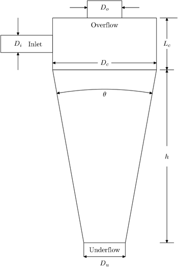
The user defines all of the cyclone dimensions and the model then calculates the d₅₀ in microns, the pressure drop across the cyclone and the liquid distribution between the over and under flows.

The following equations are used to determine the cyclone operation⁴:

(7) d₅₀ Calculation

[math]\displaystyle{ {d_{50}=F\left[\cfrac{50.5\times D_c^{0.46}D_i^{0.6}D_o^{1.21}\exp(0.063C_v)}{D_u^{0.71}h^{0.38}Q^{0.45}(\rho_s-\rho_l)^{0.5}}\right]} }[/math]

where d₅₀ is in microns

D_c- Cyclone diameter, cm

D_i - Cyclone feed inlet diameter, cm

D_o- Cyclone overflow or Vortex finder diameter, cm

D_u- Cyclone underflow or Apex diameter, cm

h - Free vortex height in cyclone, cm

Q - Volumetric flow rate of each cyclone feed at temperature,l/min

C_v - Volumetric percent of solids in feed slurry at temperature

[math]\displaystyle{ \rho_s }[/math] - Solids density at Temperature (t/m³)

[math]\displaystyle{ \rho_l }[/math] - Liquid density at Temperature (t/m³)

F - d₅₀ correction factor.

(8) Pressure Drop across the Cyclone in kPa

[math]\displaystyle{ \Delta P =PressFactor\times\cfrac{1.88Q^{1.78}\exp(0.0055C_v)} {D_{c}^{0.37}D_{i}^{0.94}h^{0.28}(D_u^2+D_o^2)^{0.87} } }[/math]

where PressFactor - Pressure drop correction factor

(9) Pressure drop across cyclone, in metres of feed slurry

[math]\displaystyle{ H=\cfrac{\Delta P}{g\rho_{Feed}} }[/math]

(10) Recovery of feed volume to the underflow product

[math]\displaystyle{ R_v=\cfrac{S}{S+1} }[/math]

where

[math]\displaystyle{ S = SFactor* \cfrac{1.9 \left(\cfrac{D_u}{D_o} \right)^{3.31}h^{0.54}(D_u^2+D_o^2)^{0.36}*exp(0.0054C_v)} {H^{0.24}D_c^{1.11}} }[/math]

where SFactor - S correction factor

(11) Sharpness Separation

_{[math]\displaystyle{ \mathbf{\mathit{m=SharpFactor*1.94*exp(-1.58*R_v)*\left(\cfrac{D_c^2*h}{Q} \right)^{0.15}}} }[/math]}

For backward compatibility when OldSharpnessCalc is selected, Plitt sharpness term is calculated as

_{[math]\displaystyle{ \mathbf{\mathit{m=SharpFactor*1.94*exp\left[(-1.58*R_v)*\left(\cfrac{D_c^2*h}{Q} \right)^{0.15}\right]}} }[/math]}

where: R_v - Recovery of feed volume to the underflow product

SharpFactor - Sharpness correction factor

Q - Volumetric flow rate of each cyclone feed at temperature, l/min

Assumptions (Plitt)

The pressure drop equation assumes free discharge from both the under and over flows from the cyclone.
The mass weighted mean of the solids density is used to determine the cut point.
Q in the sharpness equation is the total volumetric flow into the cyclones.

Nageswararao Model

The user defines all of the cyclone dimensions and the model then calculates the d₅₀ in microns, the pressure drop across the cyclone and the liquid distribution between the over and under flows.

The following equations are used to determine the cyclone operation⁵:

(12) Cyclone Throughput:

[math]\displaystyle{ {\cfrac{Q}{D_c^{2}\sqrt{P/\mathit{\rho_p}}} = K_{Qo}D_c^{-0.10} \left(\cfrac{D_o}{D_c} \right)^{0.68} \left(\cfrac{D_i}{D_c} \right)^{0.45} \left(\cfrac{L_c}{D_c} \right)^{0.20}\mathit{\Theta^{-0.10}}} }[/math]

where D_c - Cyclone diameter, cm

D_i - Cyclone feed inlet diameter, cm

D_o - Cyclone overflow or Vortex finder diameter, cm

K_Qo - Material dependent constant for performance characteristic, P_i

L_c - Length of the cylindrical section of the cyclone, cm

P - Cyclone feed pressure, kPa

Q - Cyclone throughput, l/min

[math]\displaystyle{ \mathbf{\mathit{\Theta}} }[/math] - full cone angle, degrees

(13) d_50c Calculation

[math]\displaystyle{ {\cfrac{d_{50c}}{D_c}=K_{Do} \left(D_c^{-0.65} \right) \left(\cfrac{D_o}{D_c} \right)^{0.52} \left(\cfrac{D_u}{D_c}\right)^{-0.50} \left(\cfrac{D_i}{D_c}\right)^{0.20} \left(\cfrac{L_c}{D_c} \right)^{0.20}\mathit{\Theta^{0.15}} \left(\cfrac{P}{\mathit{\rho_p}gD_c} \right)^{-0.22}\mathit{\lambda^{0.93}}} }[/math]

where d_50c is the corrected cut size in microns

D_u - Cyclone underflow or spigot diameter, cm

g - acceleration due to gravity, m/s²

K_Do - Material dependent constant for performance characteristic, P_i

[math]\displaystyle{ \rho_p }[/math] - Density of feed pulp, (t/m³)

[math]\displaystyle{ \lambda }[/math] - hindered settling factor

Nageswararao Hindered Settling Factor:

[math]\displaystyle{ {\lambda = \cfrac{10^{1.82C_v}}{8.05\times(1-C_v)^{2}}} }[/math]

Richardson Zaki Settling Factor:

[math]\displaystyle{ {\lambda = (1-C_v)^{2.39}} }[/math]

C_v - Volumetric fraction of feed solids.

(14) Recovery of water to the underflow product

[math]\displaystyle{ {R_f = K_{Wo}\left(D_c^{-0.00}\right)\left(\cfrac{D_o}{D_c}\right)^{-1.19}\left(\frac{D_u}{D_c}\right)^{2.40}\left(\cfrac{D_i}{D_c}\right)^{-0.50} \left(\cfrac{L_c}{D_c}\right)^{0.22} \mathit{\Theta^{-0.24}}\left(\cfrac{P}{\mathit{\rho_p}gD_c}\right)^{-0.53}\mathit{\lambda^{0.27}}} }[/math]

where K_Wo - Material dependant constant for performance characteristic, P_i

Assumptions (Nageswararao)

The pressure drop equation assumes free discharge from both the under and over flows from the cyclone.
The mass weighted mean of the solids density is used to determine the cut point.
Q is the total volumetric flow into the cyclones.

Efficiency Curves

If the user selects the User d₅₀, Krebs, Plitt or Nageswararao models, they may choose the Efficiency Curve equation that will be used to calculate the solids size distribution across the cyclone.

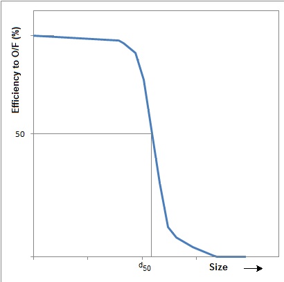
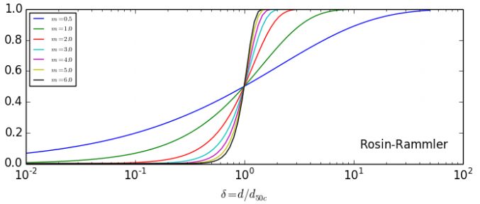
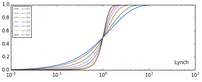
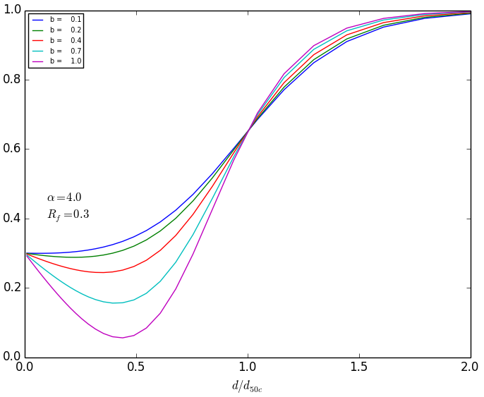
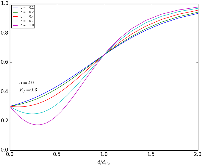
The common forms of the Efficiency Curves are the Rosin-Rammler and Lynch curves. However, these have the disadvantage of not being able to model the "fishhook" since they are monotonic. Each has a single "sharpness" parameter - as the sharpness increases, the separation about the d₅₀ increases. (d₅₀ is the size which will report with equal probability to underflow or overflow, and refers to the corrected value.)

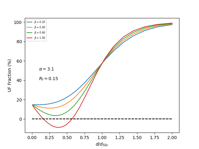
The Whiten Fishhook Efficiency curve has 2 further parameters that allow it to model the "fishhook". Furthermore, this method models the actual recovery, rather than the corrected recovery.

Note that the efficiency curve is not the actual recovery curve (the split between underflow and overflow). Hydrocyclone models assume that the fine particles do not separate, so that they effectively partition with the liquid, so that the recovery for fine particles is the same as the liquid split [math]\displaystyle{ R_f }[/math]. This means that the recovery curve is related to the efficiency curve by [math]\displaystyle{ {{y=y'+R_f(1-y')}} }[/math]

Rosin-Rammler

(15) Recovery to underflow on a corrected basis for the size interval. This method is based on a Rosin-Rammler type of function with the efficiency curve expression derived by Reid and Plitt.

[math]\displaystyle{ {y_i'=1-\exp\left[-0.693147\times\left(\cfrac{d_i}{d_{50}}\right)^m\right]} }[/math]

where di - geometric mean of the size interval

m - measure of the sharpness of separation.

Lynch

(16) Recovery to underflow on a corrected basis for the size interval

[math]\displaystyle{ {{y_i'=\cfrac{\exp\left(\alpha d_i/d_{50}\right)-1}{\exp\left(\alpha d_i/d_{50}\right)+\exp(\alpha)-2}}} }[/math]

where: d_i - geometric mean of the size interval

[math]\displaystyle{ {\alpha} }[/math] = measure of the sharpness of separation

(17) The actual recovery to the underflow, y, is then calculated using the same equation for both of the above methods:

[math]\displaystyle{ {{y=y'+R_f(1-y')}} }[/math]

where R_f = fraction of feed liquid reporting to the underflow product.

Whiten Fishhook

The Whiten Fishhook curve has further parameters that allow it to model the "fishhook".

(18) This is the actual rather than corrected curve:

[math]\displaystyle{ y_i=1 - \cfrac{\exp({\alpha})-1}{\exp \left(\alpha \beta^{*} \cfrac{d_i}{d_{50}} \right) + \exp ({\alpha})-2} \left(1+{\beta}{\beta^{*}} \cfrac{d_i}{d_{50}}\right) }[/math]

where: d_i - geometric mean of the size interval

[math]\displaystyle{ \alpha }[/math] determines the slope at the larger values of d.

[math]\displaystyle{ \beta }[/math] controls the initial rise in the curve at fine sizes..

[math]\displaystyle{ \beta^* }[/math] preserves the definition of d₅₀.

Notes

The existence of the "fishhook" - where the recovery to underflow of solids initially decreases as the particle size increases - has been contentious until recently [6]; and the exact mechanisms are still uncertain. It is accepted as real now, but it is a subtle effect. If the underflow liquid recovery is too low in the SysCAD model, the fishhook effect may result in all solids in some size range report to the overflow (zero recovery) which is physically unrealistic. SysCAD will in this case set the PSD fractions to zero over this range, and report a warning that the underflow solids fraction is not achieved. In this case, either reduce the fishhook parameter [math]\displaystyle{ \beta }[/math] or the specified underflow solids.

User Curve

The user may give actual curve data to specify the solids split. Either the actual or the corrected split may be specified. This is useful in several situations:

The user may have plant data, which they want to use to tune a particular model. Also, there are other efficiency curve models not presently implemented in SysCAD, such as the Cilliers model. The user could then calculate the solids partition using a PGM, or externally and supply this to the model.

Note that specifying the curve data effectively determines the d50 for the solids split. Some of the methods such as the Nagaswararo cyclone calculate the d50 - it is up to the user to ensure that the d50 for the specified split is equal to that calculated by the model (or at least understand that they are using a different d50.) SysCAD will display the d50 for the user curves, and this can be compared to the calculated d50.

References

R.A.Arterburn, The Sizing and Selection of Hydrocyclones, Metallurgical Handbook.
D.T.Tarr, Practical application of liquid cyclones in mineral dressing problems, Krebs Engineers documentation, October 1965.
L.R.Plitt, A mathematical model of the hydrocyclone classifier, CIM Bulletin, December 1976.
T.P.Napier-Munn, Mineral Comminution Circuits: Their Operation and Optimisation, JKMRC Monograph Series in Mining and Mineral Processing 2, 1999.
K. Nageswararao, D.M. Wiseman, T.J. Napier-Munn, Two empirical hydrocyclone models revisited, Minerals Engineering 17 671–687, 2004.
Florent Bourgeois, Arun K. Majumder, Is the fish-hook effect in hydrocyclones a real phenomenon?, Powder Technology, Volume 237, 2013

Data Sections

The default sections and variable names are described in detail in the following tables. The default Hydrocyclone access window consists of 5 sections. This number may increase, based on user configuration.

Summary of Data Sections

Hydrocyclone tab - Allows the user to select the Hydrocyclone method and displays a summary of the flows in the Feed, Overflow and Underflow streams.
Cyclone tab - This page contains all of the fields relating to the Hydrocyclone method.
PartCrv tab - This tab displays the partition curve data for the cyclone.
QFeed - Optional tab, only visible if ShowQFeed is enabled. This page shows the properties of the mixed stream as the feed to the Hydrocyclone model.
QOFlow - Optional tab, only visible if ShowQOFlow is enabled. This page shows the properties of the overflow stream from the Hydrocyclone model.
QUFlow - Optional tab, only visible if ShowQUFlow is enabled. This page shows the properties of the underflow stream from the Hydrocyclone model.
Info tab - Contains general settings for the unit and allows the user to include documentation about the unit and create Hyperlinks to external documents.
Links tab, contains a summary table for all the input and output streams.
Audit tab - Contains summary information required for Mass and Energy balance. See Model Examples for enthalpy calculation Examples.

Hydrocyclone Page

Unit Type: Hydrocyclone - The first tab page in the access window will have this name.

Tag (Long/Short)	Input / Calc	Description/Calculated Variables / Options
Tag	Display	This name tag may be modified with the change tag option.
Condition	Display	OK if no errors/warnings, otherwise lists errors/warnings.
ConditionCount	Display	The current number of errors/warnings. If condition is OK, returns 0.
GeneralDescription / GenDesc	Display	This is an automatically generated description for the unit. If the user has entered text in the 'EqpDesc' field on the Info tab (see below), this will be displayed here. If this field is blank, then SysCAD will display the UnitType or SubClass.
Requirements
On	Tickbox	This allows the user to Enable or Disable the unit. If the Hydrocyclone is disabled (turned OFF), then all of the material will flow out of the underflow stream.
Method	Simple (no PSD)	The unit does not use, or require, the Size Distribution information to calculate solids split. The user defines the solids and liquids split on a simple mass fraction basis.
	User Defined Curves	The user specifies an Efficiency Curve (or partition curve) on the Partition Curve page, which is used to calculate the separation of the solids. The user also specifies the fraction of solids in the Cyclone underflow. The model calculates the Actual d₅₀ of the cyclone and the liquid split to the under and over flows.
	User d50	The user specifies the actual d₅₀ of the cyclone, the required Efficiency Curve Split Method and the percent solids in the underflow.
	Krebs Cyclone	The unit uses the Krebs Cyclone Model to calculate the operating parameters of the cyclone. The user specifies the cyclone diameter and, the percent solids in the underflow and the required Efficiency Curve Split Method. The model calculates the d₅₀ of the cyclone. The feed solids volume concentration must be greater than 53% to use this method.
	Plitt Cyclone	The unit uses the Plitt Cyclone Model to calculate the operating parameters of the cyclone. The user specifies the all of the physical parameters of the cyclone and the required Efficiency Curve Split Method. The model calculates the d₅₀ of the cyclone and the liquid split to the under and over flows.
	Nageswararao	The unit uses the Nageswararao Model to calculate the operating parameters of the cyclone. The user specifies the all of the physical parameters of the cyclone and the required Efficiency Curve Split Method. The model calculates the d₅₀ of the cyclone and the liquid split to the under and over flows.
Predictive Models for which all properties are calculated.
Options
ShowQFeed	Tickbox	Allows the user to display the properties of the feed streams to the Cyclone is a single Feed stream.
ShowQOFlow	Tickbox	Allows the user to display the properties of the overflow streams from the Cyclone.
ShowQUFlow	Tickbox	Allows the user to display the properties of the underflow streams from the Cyclone.
SizeForPassingFracCalc	Input	The particle size to be used for the percent 'Passing' display for ALL units in the Project.
FracForPassesSizeCalc	Input	The fraction percent passing to be used for the 'Passes' display for ALL units in the Project.
Intervals		The user may toggle between displaying the size intervals ascending or descending.
Results
DistributionUsed	Display	Displays the size distribution used. (useful for projects containing multiple size distributions)
Stream Result Summary This table shows the following variables for the Feed, Underflow and Overflow streams.
MassFlow / Qm	Display	The total mass flow in each stream.
SolidMassFlow / SQm	Display	The Solids mass flow in each stream.
LiquidMassFlow / LQm	Display	The Liquid mass flow in each stream.
VolFlow / Qv	Display	The total Volume flow in each stream.
Temperature / T	Display	The Temperature of each stream.
Density / Rho	Display	The Density of each stream.
SolidFrac / Sf	Display	The Solid Fraction in each stream.
LiquidFrac / Lf	Display	The Liquid Fraction in each stream.
Passing	Display	The mass fraction passing the user specifies size (in the field 'SizeForPassingFracCalc') in each stream.
Passes	Display	The user specified (in the field 'FracForPassesSizeCalc') fraction of material in each stream will pass this size fraction.

Cyclone Page

Tag (Long/Short)	Input / Calc	Description/Calculated Variables / Options
Requirements
CyclonesCount	Input	The number of cyclones in the bank. This allows the user to emulate a bank of cyclones in a single unit. For the 'User Defined Curves' and 'User d50' methods, the number of cyclones is only used to calculate the flow per cyclone. This field is not visible if the user has chosen Method = 'Simple'.
The parameters in the access window change depending on the cyclone model chosen by the user. The input parameters for each model will be detailed separately below. Where a model has output parameters that are only displayed for that particular model, these are also shown individually. The Results fields that are common to all methods are shown in the Common Results section.
Simple (no PSD)
UFSolidsMethod	UF Solids Fraction	The user may set the required fraction of solids in the cyclone underflow.
UFSolidsMethod	UF Solids Conc25	The user may set the required concentration of solids in the cyclone underflow at 25°C.
UFSolidFracReqd	Input	Only visible if the UF Solids Fraction method has been chosen. The required mass fraction of solids in the cyclone Underflow stream.
UFSolidConc25Reqd	Input	Only visible if the UF Solids Conc25 method has been chosen. The required concentration of solids in the cyclone Underflow stream at 25°C.
RecoveryMethod	Liquid Recovery R_f
	Slurry Recovery R_v	The user may set the required volume recovery of slurry from the Feed stream to the cyclone underflow.
	Solids Mass Recovery	The user may set the required mass recovery of solids from the Feed stream to the cyclone underflow.
	Solids Volume Recovery	The user may set the required volume recovery of solids from the Feed stream to the cyclone underflow.
LiquidRecoveryReqd / RfReqd	Input	Only visible if the Liquid Recovery R_f method has been chosen. The required mass fraction of the Feed liquids that must report to the cyclone Underflow stream.
SlurryRecovery / dRv	Input	Only visible if the Slurry Recovery R_v method has been chosen. The required mass fraction of the Feed slurry that must report to the cyclone Underflow stream.
SolidsMassRecovery / dRsm	Input	Only visible if the Solids Mass Recovery method has been chosen. The required mass fraction of the Feed solids that must report to the cyclone Underflow stream.
SolidsVolRecovery / dRs	Input	Only visible if the Solids Volume Recovery method has been chosen. The required volume fraction of the Feed solids that must report to the cyclone Underflow stream.
Results
UF.SolidFrac / UF.Sf	Display	The mass fraction of solids in the cyclone Underflow stream.
UF.SolidConc25	Display	The concentration of solids in the cyclone Underflow stream at 25°C.
Please see Common Input Fields for a description of the Selected Solid Species Calculation Method inputs.
Specification
User Defined Curves
The user will also see a tab 'PartCrv' where they must enter the fraction of each size interval reporting to the cyclone underflow. An example of an Efficiency Curve is shown in Efficiency Curve Theory. Please see Common Input Fields for a description of the Underflow Requirements and Selected Solid Species Calculation Method inputs.
User d50
CutSizeReqd / d50Reqd	Input	The required d₅₀ of the cyclone.
Please see Common Input Fields for a description of the Underflow Requirements, Efficiency Curve and Selected Solid Species Calculation Method inputs.
Krebs Cyclone
(The feed solids volume concentration must be greater than 53% to use this method.)
CycloneDiameter / Dc	Input	The diameter of the cyclone.
Kr.Factor	Input	This is the correction factor to account for differences in the cyclone geometry from the 'optimum' dimensions. This is used to adjust the calculated cut point of the cyclone. The default value is 1. (See Equation (1) in the Krebs theory)
PressChange / dP	Display	The calculated pressure drop across the cyclone.
Please see Common Input Fields for a description of the Underflow Requirements, Efficiency Curve and Selected Solid Species Calculation Method inputs.
Plitt Cyclone
Cyclone Geometry
CycloneDiameter / Dc	Input	The diameter of the cyclone.
InletDiameter / Di	Input	The inside diameter of the cyclone feed inlet.
VortexDiameter / Do	Input	The inside diameter of the overflow or the vortex finder.
SpigotDiameter / Du	Input	The inside diameter of the underflow or the spigot diameter.
Height / h	Input	The free vortex height of the cyclone, defined as the distance from the bottom of the vortex finder to the top of the underflow orifice. h = Total length of the cyclone - vortex length
Correction Factors
d50Factor	Input	This Factor is used to adjust the d₅₀ of the cyclone. Increasing this value will increase the d₅₀ used in the calculations, and hence increase the amount of solids reporting to the cyclone Overflow. Please see Equation (7) in the Plitt Model Theory.
SharpFactor	Input	Sharpness Factor is used to adjust "m". Increasing this value will increase the sharpness of separation and more of the coarse particles will report to the underflow. Please see Equation (11) in the Plitt Model Theory.
PressFactor	Input	Press Factor is used to adjust "dP". Increasing this value will increase the pressure drop across the cyclone and hence change the size recovery of the cyclone. Please see Equation (8) in the Plitt Model Theory.
SFactor	Input	SFactor is used to adjust "S", which influences the recovery of feed volume to the cyclone underflow. Increasing this value will increase the recovery to the cyclone underflow. Please see Equation (10) in the Plitt Model Theory.
OldSharpnessCalc	Tickbox	Only available in Build 138.27040 or later. If ticked, the original (incorrect) calculation for sharpness will be used. If unticked (recommended), the correct calculation will be used for the sharpness calculation.
OverrideSharpness	Tickbox	If ticked, this will enable the user to override the calculated Sharpness parameter. (in earlier builds (before 138.27040) this parameter is shown further down the page).
Please see Common Input Fields for a description of the Efficiency Curve and Selected Solid Species Calculation Method inputs.
Results
CutSize / d50	Display	The calculated d₅₀ of the cyclone.
PressChange / dP	Display	The calculated pressure drop across the cyclone.
FeedSolidsVolFrac / Cv	Display	The calculated solids fraction in the feed by volume.
VolFlowSplit / S	Display	The calculated ratio of the underflow volumetric flow to the overflow volumetric flow. Please see Equation (10) in the Plitt Model Theory.
VolRecovery / Rv	Display	Recovery of feed volume to the underflow.
SolidsRecovery / Rs	Display	Recovery of feed solids to the underflow.
Bypass / dRf	Display
RRSharpness / m	Display	The calculated efficiency exponent in Rosin-Rammler efficiency curve. This is a measure of the sharpness of separation of the cyclone.
LynchSharpness / alpha	Display	The calculated alpha term for the Lynch sharpness equation.
Nageswararao
HinderingCalc	Nageswararao	The Nageswararao Hindered Settling Factor will be used. Please refer to Nageswararao Model Theory for more information.
HinderingCalc	Richardson-Zaki	The Richardson Zaki Settling Factor will be used. Please refer to Nageswararao Model Theory for more information.
Cyclone Geometry
CycloneDiameter / Dc	Input	The diameter of the cyclone.
InletDiameter / Di	Input	The inside diameter of the cyclone feed inlet.
VortexDiameter / Do	Input	The inside diameter of the overflow or the vortex finder.
SpigotDiameter / Du	Input	The inside diameter of the underflow or the spigot diameter.
CylSectLength / Lc	Input	The length of the cylindrical section of the cyclone.
FullConeAngle / theta	Input	The angle of the cyclone cone.
Material Constants
KQ0	Input
Kd0	Input	Material dependent constant for performance characteristic, Pi.
KW0	Input	Material dependent constant for performance characteristic, Pi.
KV0	Input
Please see Common Input Fields for a description of the Efficiency Curve and Selected Solid Species Calculation Method inputs.
Dimensionless Results
EulerNumber / EU	Display
EulerFroude / EF	Display	Product of Euler and Froude numbers.
HinderedSettling / lambda	Display	Hindered settling factor, a function of the volumetric fraction of feed solids (FeedSolidsVolFrac/Cv). Used in equation 13, see Nageswararao Model Theory for more details.
Stream Dependent Results
FeedSolidsVolFrac / Cv	Display	The calculated solids fraction in the feed by volume.
FeedVolFlow / Q	Display	Feed volume flow per cyclone.
PressChange / dP	Display	The calculated pressure drop across the cyclone.
SlurryDensity / RhoP	Display	The density of the feed slurry.
InletVelocity / Vi	Display	Inlet velocity.
CycloneVelocity / Vc	Display	Cyclone velocity.
Recovery
d50	Display	The calculated d₅₀ of the cyclone.
ActualRecovery / Rf	Display	Recovery of water to the underflow.
VolRecovery / Rv	Display	Recovery of feed volume to the underflow.
RfW	Display
RfV	Display
Common Input Fields
The following 3 fields are visible for the 'simple' cyclone methods - User Defined Curves, User d50 and Krebs Cyclone methods.
UnderflowConc	Tickbox	If this box is ticked it allows the user to set the solids in the underflow as a concentration at 25°C. Otherwise the user sets the fraction of solids in the underflow.
UFSolidFracReqd	Input	The user sets percentage of solids in the cyclone underflow. This field is only visible if 'UnderflowConc' is NOT ticked.
UFSolidConc25Reqd	Input	The required concentration of solids in the cyclone underflow at 25°C. This field is only visible if 'UnderflowConc' is ticked.
The following field is visible for the all cyclone methods. (only available in Build 138 or later)
VapourToUF	Input	The required fraction of vapours in the feed that will pass to the underflow stream. The rest will pass to the overflow stream.
The following fields are visible for most of the cyclone methods.
Efficiency Curve
SplitMethod	Rosin-Ramler	The Rosin-Rammler method is used to calculate the solids split in each size interval.
	Lynch	The Lynch method is used to calculate the solids split in each size interval.
	Whiten Fishhook	The Whiten-Fishhook method is used to calculate the solids split in each size interval.
	User Curve	The user can define their own partition curve.
Sharpness / m	Input	Only visible if the Rosin-Ramler method has been chosen. The required sharpness value. For Plitt model when OverrideSharpness is not selected then this is calculated by Plitt model.
SharpnessFactor / Alpha	Input	Only visible if the Lynch or Whiten-Fishhook methods have been chosen. The required sharpness factor or Alpha value. For Plitt model when OverrideSharpness is not selected then this is calculated by Plitt model.
Fishhook / Beta	Input	Only visible if the Whiten-Fishhook method has been chosen. The required Beta value used in the Whiten-Fishhook equation.
Beta*	Display	Only visible if the Whiten-Fishhook method has been chosen. The calculated Beta* value used in the Whiten-Fishhook equation.
SolSp...
Selected Solid Species Calculation Method - Please see Example Solid Species (bypass) calculation for sample calculation.
ShowSelectedSolids	Tickbox	If ticked, allows user to override calculated solid splits for specific solid species.
Count	Input	Only visible if ShowSelectedSolids has been ticked. The number of solid species for which the user wishes to override the calculated solid splits.
SpeciesX	List	The number of these fields will be equal to Count. The user can choose a specific solid species from the list of all solid species in the project.
For each selected species the following parameters are displayed
WithLiq	Input	The fraction of the selected solid species which will follow the liquid split.
To UF	Input	The fraction of the selected solid species which will report directly to the underflow.
To OF	Input	The fraction of the selected solid species which will report directly to the overflow.
WithSol	Display	The fraction of the selected solid species which will follow the solid split. If using multiple solid species with size definition, please see notes under Example Solid Species (bypass) calculation for more information.
Common Data Fields
Actual Results
The following field is visible for the User d50 and Krebs Cyclone method.
CutSize / d50	Display	The calculated d₅₀ of the cyclone.
The following 5 fields are visible for the User Defined Curves, User d50 and Krebs Cyclone methods.
UF.SolidFrac / UF.Sf	Display	The fraction of solids in the cyclone underflow stream.
UF.SolidConc25	Display	The solids concentration at 25°C in the cyclone underflow stream.
FeedSolidsVolFrac / Cv	Display	The calculated solids fraction in the feed by volume.
LiquidRecovery / Rf	Display	The fraction of liquids in the feed reporting to the underflow stream.
SlurryRecovery / Rv	Display	The volume fraction of slurry in the feed reporting to the underflow stream.
SolidsRecovery / Rs	Display	The fraction of solids in the feed reporting to the underflow stream.
The following 4 fields are visible for the Simple (no PSD) and Plitt methods.
Recoveries
ActualVolumeRecovery / ActRv	Display	The volume fraction of slurry in the feed reporting to the underflow stream.
ActualLiquidRecovery / ActRf	Display	The fraction of liquids in the feed reporting to the underflow stream.
ActualSolidsRecovery / ActRs	Display	The fraction of solids in the feed reporting to the underflow stream.
ActualSolidMassRecovery / ActRsm	Display	The mass fraction of solids in the feed reporting to the underflow stream.

Partition Curve Page

The Hydrocyclone has a section showing the partition curve. This page is displayed if the User Defined Curves, User d50, Krebs Cyclone or Nageswararao methods are chosen.

The model will calculate the partition curve for the Hydrocyclone configuration and display it on this page.

Tag (Long/Short)	Input or Calc	Description
Efficiency Curve
CorrectedCurve	Tickbox	Only visible if the User Defined Curves method or User Curve SplitMethod has been chosen. If ticked, allows to user to set the Corrected Partition Curve, which is applied directly to the solids separation. If not ticked, the user enters the Actual Partition Curve which is "corrected" prior to being applied to the solids separation.
For each size interval, the following fields are shown.
Corrected	Input/Display	This will be an input field if the User Defined Curves method or User Curve SplitMethod has been chosen and the CorrectedCurve box has been ticked. The partition curve applied to the solids separation.
Actual	Input/Display	This will be an input field if the User Defined Curves method or User Curve SplitMethod has been chosen and the CorrectedCurve box has NOT been ticked. The desired partition curve prior to "correction".

Example Solid Species (bypass) calculation

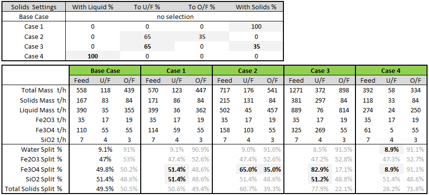
Below is an example from the Milling and Magnetic Separation Example, looking at the behaviour of Prim_Mill_Cyc.

In this example, the feed to the cyclone contain 3 species (Fe2O3, Fe3O4 and SiO2) with size distribution data defined (caused by different recovery values from the Rough_Mag_Sep).
We will look at how the solids recovery is affected when we select one species to split differently using the SolSp section.
Five sample calculations were completed, note that the feed to the cyclone is not constant as underflow is being recirculated back to the cyclone feed.
An example species selection and species split setting is given below, this matches Case 2 in the table given below:

Sample Data Setting and Calculated Results.

NOTES:

Solid Species Split are calculated as follows:
- If a solid species has its own size distribution defined, then the solid species will split based on its size data.
- If solid species have no individual size distribution data defined (let's call these solids the remaining solids), then the remaining solids will follow the same split as the species with size distribution defined.
- If multiple species have size distribution defined, then the remaining solids will follow the same split as LAST species with size distribution defined. In our example, this species is SiO2.
If a solid species is selected using the "SolSp" Option, then this will override its defined size distribution data, if any, and follow the split method defined in the SolSp section.
- Case 1: Fe3O4 ignores its size distribution definition, and follows the size distribution as per remaining solids. (With Sol = follow SiO2 Split)
- Case 2: Fe3O4 ignores its size distribution definition, and splits 65% to U/F and 35% to O/F.
- Case 3: Fe3O4 ignores its size distribution definition, and splits 65% straight to U/F, the other 35% follows the same split as remaining solids. So the total species split to underflow is 65% + 35% * SiO2 Split = 65 + 35 * 0.51 = 83%.
- Case 4: Fe3O4 ignores its size distribution definition, and follows the split as per liquid split.

Adding this Model to a Project

Add to Configuration File

Sort either by DLL or Group:

	DLL:	Separation.dll	→	Units/Links	→	Size Separation: Hydrocyclone
or	Group:	Size Distribution	→	Units/Links	→	Size Separation: Hydrocyclone

See Model Selection for more information on adding models to the configuration file.

Insert into Project Flowsheet

Insert Unit

→

Size Separation

→

Hydrocyclone

See Insert Unit for general information on inserting units.

Hydrocyclone

Contents